SciELO - Scientific Electronic Library Online

 
vol.8 número2UNA ESPECIE NUEVA DE FURCRAEA (AGAVACEAE) DE COLOMBIATELMATOBLECHNUM (BLECHNACEAE): A NEW GENUS FOR THE URUGUAYANFLORA índice de autoresíndice de materiabúsqueda de artículos
Home Pagelista alfabética de revistas  

Servicios Personalizados

Revista

Articulo

Indicadores

  • No hay articulos citadosCitado por SciELO

Links relacionados

Compartir


Darwiniana, nueva serie

versión impresa ISSN 0011-6793versión On-line ISSN 1850-1699

Darwiniana, nueva serie vol.8 no.2 San Isidro dic. 2020

http://dx.doi.org/10.14522/darwiniana.2020.82.894 

Sistemática y taxonomía de Plantas

DISTRIBUTION MODELS AND MORPHOMETRIC ANALYSES AS ADDITIONAL TOOLS FOR THE STUDY OF DIVERSIFICATION IN DEYEUXIA VELUTINA, AN ANDEAN GRASS SPECIES

María A. Ferrero11 

Agostina B. Sassone2,32  3 

Liliana M. Giussani22 

Andrea S. Vega1 

1 Universidad de Buenos Aires, Facultad de Agronomía, Departamento de Recursos Naturales y Ambiente, Cátedra de Botánica General, Av. San Martín 4453, C1417DSE, Buenos Aires, Argentina; mferrero@agro.uba.ar (author for correspondence).

2 Instituto de Botánica Darwinion, Labardén 200, San Isidro, B1642HYD, Buenos Aires, Argentina.

3 Leibniz Institute of Plant Genetics and Crop Plant Research (IPK), Corrensstraße 3, 06466 Gatersleben, Germany.

Resumen

Ferrero, M. A.; A. B. Sassone, L. M. Giussani & A. S. Vega. 2020. Modelos de distribución y análisis morfométrico en Deyeuxia velutina, una especie andina de gramínea. Darwiniana, nueva serie 8(2): 509-524.

Rúgolo de Agrasar reconoció dos variedades de Deyeuxia velutina (D. velutina var. velutina y D. velutina var. nardifolia) basándose en el indumento de las vainas, la longitud de la lemma, y la dirección de las hojas. Sin embargo, su delimitación taxonómica ha sido dificultosa debido a la superposición ocasional de estos caracteres. A fin de evaluar la delimitación infraespecífica de D. velutina, presentamos un estudio exhaustivo que combina análisis morfométrico y modelos de distribución potencial. Para explorar la variación morfológica y seleccionar caracteres diagnósticos, medimos 124 caracteres morfológicos en 52 especímenes de ambas variedades y realizamos un Análisis de Coordenadas Principales y análisis univariados (análisis de la varianza y la prueba no paramétrica de Kruskal- Wallis). Ambos taxones resolvieron como grupos morfológicos definidos. Adicionalmente, se realizó un análisis discriminante para clasificar los individuos en los grupos morfológicos predeterminados.

Con el fin de modelar la distribución de la especie, se georreferenciaron 26 especímenes de D. velutina var. nardifolia y 68 de D. velutina var. velutina y se analizaron 20 variables ambientales a través del Modelo de Máxima Entropía. Deyeuxia velutina se extiende en regiones altoandinas desde Perú hasta el sur de Argentina y Chile. Ambas variedades difieren en su distribución geográfica; el análisis de regresión de la latitud y longitud en relación con las coordenadas principales del PCoA confirmó esta diferenciación. Deyeuxia velutina var. nardifolia está restringida a la zona norte de la distribución, mientras que D. velutina var. velutina mostró mayor probabilidad de presencia en la región sur. Por otra parte, D. velutina var. nardifolia es reportada aquí por primera vez en la provincia de San Juan (Argentina), lo que constituye el límite austral de su distribución geográfica. Se consideraron caracteres morfológicos adicionales en una clave actualizada de las variedades.

Keywords: Diagnostic characters; geographical patterns; morphometry; integrative taxonomy.

Abstract

Ferrero, M. A.; A. B. Sassone, L. M. Giussani & A. S. Vega. 2020. Distribution models and morphometric analyses in Deyeuxia velutina, an Andean grass species. Darwiniana, nueva serie 8(2): 509-524.

Rúgolo de Agrasar recognized two varieties of Deyeuxia velutina (D. velutina var. velutina and D. velutina var. nardifolia) based on leaf sheath indumentum, lemma length, and leaf blade direction. However, taxonomic delimitation has been difficult due to occasional overlapping characters. To assess the infraspecific delimitation of D. velutina, we present a comprehensive study combining morphometric analyses and a potential distribution model. To explore morphological variation and select diagnostic characters, we measured 124 morphological characters in 52 specimens of both varieties and performed a principal coordinate analysis and univariate analyses (Analysis of variance and Kruskal-Wallis non- parametric test). Both taxa resolved as separate morphological groups. Additionally, a Discriminant Analysis was performed to classify the individuals in the predetermined morphological groups. For modeling the species distribution, 26 specimens of D. velutina var. nardifolia and 68 of D. velutina var. velutina were georeferenced and 20 environmental variables were analyzed through a Maximum Entropy model. Deyeuxia velutina extends in the high Andean region from Peru to southern Argentina and Chile. Both varieties differed in their geographical limits, a result supported by regression analyses of latitude and longitude on the principal coordinates of the PCoA. Deyeuxia velutina var. nardifolia is restricted to the northern area of distribution while D. velutina var. velutina showed a higher habitat suitability in the southern region. Moreover, D. velutina var. nardifolia is here reported for the first time in San Juan province (Argentina), constituting the austral limit of its geographical distribution. Additional reliable morphological characters were considered in an updated key to the varieties.

Keywords: Diagnostic characters; geographical patterns; morphometry; integrative taxonomy.

INTRODUCTION

Deyeuxia Clarion ex P. Beauv. (Poaceae) is one of the richest genera of native grass species in South America (Rúgolo de Agrasar, 2006) and the Andes are its center of diversification. The validity of this genus is still under discussion. According to a recent treatment, most of the South American species of Deyeuxia within the Koeleriinae clade B of the Aveninae J. Presl (Saarela et al., 2017) has been transferred to the genus Cinnagrostis Griseb. (Peterson et al., 2019). Their taxonomical decision was based on a molecular phylogeny that considers three plastid and one nuclear DNA regions though the type species C. polygama Griseb. had not been included (Saarela et al., 2017); also, they considered for this decision an unpublished study of Romaschenko et al. (Peterson et al., 2019). Furthermore, new combinations and the establishment of new genera were based on weakly supported clades (Saarela et al. 2017). On this basis, we decided to maintain the validity of the genus Deyeuxia.

Endemism is commonly found within Deyeuxia (Rúgolo de Agrasar, 2006). This genus is characteristic of the “Altoandina” phytogeographic province (Weberbauer, 1945; Cabrera, 1957). The weather is cold throughout the year, and snow and hail are the most common type of precipitation being less than 400 mm annually. In this harsh environment, xerophytic grasses and cushioned or crawling dicotyledons are prevalent. The vegetation is poor and Deyeuxia is mentioned as a characteristic grass of this province (Cabrera, 1978).

Deyeuxia velutina Nees & Meyen is a native species that inhabits high elevation areas of the Andes (Peru, Bolivia, Chile, and Northwestern Argentina; Rúgolo de Agrasar, 2006; Villavicencio & Rúgolo, 2014). The presence of this species in Peru and Bolivia is based on only one specimen of each country [the type specimen of D. scabriuscula Wedd., a synonym of D. velutina var. nardifolia (Weddell 441, P; Rúgolo de Agrasar, 2006) and Ruthsatz & Vogt 10507 (LPB), Villavicencio & Rúgolo, 2014, respectively]. Deyeuxia velutina has only been considered in a molecular phylogenetic study based on plastid and nuclear markers (Saarela et al., 2017). These authors found that D. velutina specimens were grouped in a clade with low support along with other taxa of Deyeuxia [D. breviaristata Wedd., D. brevifolia J. Presl, D. cabrerae (Parodi) Parodi, D. chrysophylla Phil., D. curvula Wedd., D. deserticola Phil., D. fiebrigii (Pilg.) Rúgolo, D. filifolia Wedd., D. malamalensis (Hack.) Parodi, D. trichodonta Wedd. and D. violacea Wedd.].

Based on Rúgolo de Agrasar (2006), two varieties of D. velutina were recognized: D. velutina var. velutina and D. velutina var. nardifolia (Griseb.) Rúgolo, which were differentiated by the following characters: the upper leaf sheath indumentum (dense pubescence vs. glabrous), floret length [3-4.5 (-5.5) vs. 5-5.5 mm], and leaf blade shape (flexuous, unusually straight vs. curved), respectively. The varieties grow in humid meadows but differ in their altitudinal occurrence along the Andean distribution range. Deyeuxia velutina var. nardifolia grows along central Andean mountains of Peru, Bolivia, Chile, and northwestern Argentina at 3200-5000 m a.s.l. (Rúgolo de Agrasar, 2006; 2009; Rúgolo, 2012; Villavicencio & Rúgolo, 2014). On the other hand, D. velutina var. velutina extends along the Andean region of Chile and Argentina at 2300-4200 m a.s.l. (Rúgolo de Agrasar, 2006; 2009; Rúgolo, 2012). Nevertheless, infraspecific identification of recent collections of D. velutina varieties along the overlapping distributional range have been problematical due to ambiguous diagnostic characters.

Wiens (2011) considered that biogeographic patterns arise from dispersal limits, and species do not extend beyond their environmental niche, including abiotic and biotic factors. Therefore, differences in environmental variables (precipitation, temperature, seasonality, altitude, among others) could drive speciation since climatic-niche divergence may conduct incipient species to occupy different habitats (Hua & Wiens, 2013). These variables combined with geographical occurrences are commonly used to delimit cryptic species or species complexes through species distribution modeling analysis (e.g. Wiens & Graham, 2005; Raxworthy et al., 2007; Rissler & Apodaca, 2007; Fernández et al., 2017). This analysis is useful for studying geographic distribution and habitat preferences, aimed at species conservation and taxa delimitation (Sites & Marshall, 2003; Wiens, 2007; Schlick-Steiner et al., 2010). The combination of morphological analyses with ecological approaches may explain the influence of abiotic factors on the geographical distribution as well as their effect on specific changes in phenotypic variation patterns (Vogel Ely et al., 2018).

Traditionally, taxonomy has relied on morphological characters for the circumscription and identification of taxa. Morphometrics based on similarities (or dissimilarities) among specimens have successfully helped in delimiting groups or taxa (e.g. Sassone et al., 2013; Nicola et al., 2014; Fernández et al., 2017; Viera Barreto et al., 2018; Moroni et al., 2019). This approach and comparative studies, when considering multiple methods and independent datasets, are increasingly relevant to understand the processes that guide speciation (Sites & Marshall, 2003; Wiens, 2007; Schlick-Steiner et al., 2010).

In this contribution, we explore the morphological variability of Deyeuxia velutina varieties and its association with their geographical distribution. Our work aims to improve their delimitation through multivariate analyses and to select reliable characters from univariate analyses to provide an updated key for taxa identification. A study of species distribution model is used to map and predict the potential distribution area of the two varieties.

MATERIALS AND METHODS

Sampling

Preliminary taxa identification and character selection followed the criteria of Rúgolo de Agrasar (2006). A total of 124 morphological characters (i.e., 14 quantitative and 110 qualitative; Appendix A) were defined, coded, and added to the data matrix for analyses. Morphological data were obtained from 52 specimens (i.e., 32 of D. velutina var. velutina and 20 of D. velutina var. nardifolia; Appendix B), housed at BAA, CONC, LIL and SI herbaria (acronyms following Thiers,

2020, continuously updated).

Micromorphological studies

Florets, as well as small fragments of leaf sheaths (middle zone), were placed in glass tubes with xylene and exposed to ultrasound for approximately one hour to eliminate superficial wax and impurities. The material was air-dried, mounted, and coated with a gold-palladium (40%-60%) alloy by a Thermo VGScientific (West Sussex, UK). Photomicrographs were obtained using a Phillips XL 30 (Einhoven, The Netherlands) Scanning Electron Microscope (SEM) at the Museo Bernardino Rivadavia (Buenos Aires, Argentina).

Multivariate analyses

An ordination method was performed on standardized distance matrices (Legendre & Legendre, 1998; Oja & Paal, 2004); Principal Coordinate Analysis (PCoA) was used to analyze the morphological dissimilarity among the specimens using the Manhattan distance coefficient. A double centered matrix was employed as input to calculate eigenvectors in NTSYSpc v.2.2 (Rohlf, 1998) which were used to project the specimens in a bidimensional space. We used the packages “corrplot” (Wei & Simko, 2017) and “ggplot2” (Ginestet, 2011) in the R environment (R Core Team, 2019) for graphical representations. Finally, using a set of quantitative and non-correlated characters, a Linear Discriminant Analysis (LDA) was used to test whether morphological variation is enough to discriminate between varieties. In order to select the uncorrelated quantitative characters, we performed a Pearson’s correlation coefficient analysis using variables with r<0.5.

Table 1 Morphological quantitative characters exhibiting statistically significant differences between D. velutina 

The discrimination accuracy was evaluated using a leave-one-out cross-validation procedure to show the percentage of specimens correctly classified on the a priori groups. The LDA was performed in the R environment using the package “MASS” (Venables & Ripley, 2002).

Univariate analyses

The analysis of variance (ANOVA) and a non- parametric Kruskal-Wallis test were performed to evaluate significant differences of quantitative and qualitative variables, respectively, and to select diagnostic characters between groups as identified from the taxonomical relationships among OTUs as represented in the PCoA (Tables 1 and 2). Moreover, the Kruskal-Wallis test was also used for non-normally distributed and/or heteroscedastic characters (Nelder & Wedderburn, 1972). All statistical analyses were implemented using the package “stats” in the R environment.

Species Distribution Modeling (SDM)

Georeferences were recovered from herbaria labels of 104 specimens. After removing duplicates, the SDMs were performed with 68 specimens of D. velutina var. velutina and 26 of D. velutina var. nardifolia (Appendix B). We used the geographic coordinates [latitude (S) and longitude (W)] of the Argentinian and Chilean specimens which were obtained by the collectors using a handheld Geographical Positioning System (GPS) unit. The remaining point localities obtained from herbarium specimens were georeferenced using Google Earth 9.124.0.1 (https://earth.google.com/web). In order to avoid taxonomical and geographical errors, we carefully checked the identity of the specimens and their geographical data. We retrieved data for the 19 bioclimatic variables and altitude from WorldClim 1.4 (http://www.worldclim.com/version1), with 2.5 minutes (~5 km2) spatial resolution (Hijmans et al., 2005). We defined a rectangular area from 57° to 20° S and 72° to 52° W to calibrate our models explicitly excluding Bolivia and Peru due to scarce collections in these countries. The species distribution models were constructed using MaxEnt v.3.4.0 (Phillips et al., 2004) in the R environment through the package “dismo” (Hijmans et al., 2016). Maxent analyses were performed setting maximum iterations to 1000, and all other options were left as default (logistic output, convergence threshold of 0.00001, 10,000 background points, regularization multiplier of 1, default prevalence of 0.5 and autofeatures). We selected 70% data for training and the remaining 30% for testing. The initial model was run using the 19 bioclimatic variables and altitude. To avoid overfitting of the model we built Pearson’s correlation coefficient matrix and excluded variables (r>0.7). To decide which of the highly correlated variables should be left in the model, we used the Jackknife test of variable importance. This test provides information on the performance of each variable in the model (i.e., the importance of each variable on species distribution and the unique information it provides; Baldwin, 2009). The correlation matrix was constructed with the package “raster” (Hijmans, 2020). As a result, the final model included 6 variables for D. velutina var. velutina and 7 for D. velutina var. nardifolia, respectively (Table 3). The Area Under the Receiving Operator Characteristic curve (AUC) was used to test model’s goodness-of-fit. After calibration, we projected the results on South America.

Table 2 Mode values of morphological qualitative characters that showed significant differences between D. velutina 

Linear Regression analysis

A linear regression model was applied to measure the relationship of Axes I and II of PCoA (axes that explained most of the variability of the ordination analysis) with the geographical data (latitude and longitude). Consequently, the relationships between morphological variation and environmental changes were determined in both varieties of D. velutina. All georeferenced specimens considered in the morphometric analyses were included in the regression. The linear regression model analysis was implemented using the package “stats” in R environment (R Core Team, 2019).

RESULTS

Multivariate analyses

Sixty-one variable characters out of 124 were retained to calculate the Manhattan distance to perform Principal Coordinates (PCoA). Based on PCoA, we recognized two groups of operational taxonomic units (OTUs), corresponding to Group I and Group II (mostly in concordance with D. velutina var. nardifolia and D. velutina var. velutina, respectively). A few individuals first identified as D. velutina var. velutina (Group II) were mixed with D. velutina var. nardifolia (Group I). Both groups were mainly separated along the principal coordinate axis II (Fig. 1). Axes I and II explained 36% of the total variation.

Based on groups I and II, a Discriminant Analysis was performed using uncorrelated quantitative characters. Differences between a priori groups resulted significant (p < 0.001) on the discriminant function; the lemma length and floret width contributed most to the negative end of the linear discriminant associated with D. velutina var. nardifolia, while the inflorescence length contributed most to the positive end associated with D. velutina var. velutina. A total of 90% of the individuals were correctly classified as D. velutina var. nardifolia, while 91% were correctly classified as D. velutina var. velutina.

Fig. 1 A PCoA (Principal coordinate analyses) biplot showing the distribution of 52 OTUs based on 61 morphological characters. Groups I and II are differentiated through blue and red ellipses, respectively. Intersection of both groups shows specimens with intermediate characters. References: ● D. velutina var. velutina, ■ D. velutina var. nardifolia, ▲ specimens of D. velutina var. velutina reclassified as D. velutina var. nardifolia. Color version at http://www.ojs.darwin.edu.ar/index.php/darwiniana/article/view/894/1197 

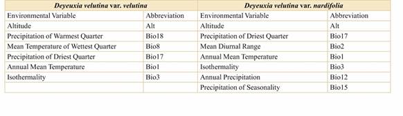
Table 3 Environmental variables used in the SDM of D. velutina var. velutina and D. velutina var. nardifolia selected from the Pearson’s correlation and Jackknife test. 

Univariate analyses

Groups as determined by multivariate analyses (PCoA and DA analyses) were tested for significant differences using ANOVA and Kruskal-Wallis tests. Univariate analyses showed differences in the height of culms, length of inflorescences, ligules and lemma, presence of hairy indumentum on the adaxial leaf blade and ligular zone, length ratio between glumes I and II, and blade apex shape (Tables 1 and 2).

An updated key to the identification of varieties is presented herein based on additional statistically significant characters; floret and leaf sheath indumentum are illustrated in Fig. 2. Quantitative characters that present overlapping ranges of variation between varieties have not been considered in the key.

1. Leaf sheath densely villous; ligular zone sericeous; ligule margin entire; leaf blade flexuous, exceptionally erect. Glumes shorter than the floret, upper glume exceptionally as long as the floret; rachilla extension ½ the length of the floret .............. D. velutina var. velutina

1. Leaf sheath glabrous; ligular zone glabrous; ligule margin denticulate, sericeous; leaf blade curved. Glumes as long as the floret; rachilla extension ¼-⅓ the length of the floret ................................ D. velutina var. nardifolia

Geographical distribution of varieties

Deyeuxia velutina inhabits high-elevation habitats along the Andes, with an altitudinal interval between 1300 to 5400 m a.s.l. The species have been reported to occur from Peru to the center of Argentina, reaching Neuquén, and our potential distribution models predict suitable environmental conditions between 8°-35° S and 68°-77° W (Fig. 3).

The species distribution models mostly reflected the known distribution of each variety. The average AUC test values of the SDM models were 0.96 and 0.97 for D. velutina var. velutina and D. velutina var. nardifolia, respectively. Although both potential distributions overlap, D. velutina var. nardifolia present a higher habitat suitability in the northern area (Fig. 3A) and D. velutina var. velutina in the southern zone of the distribution of the species (Fig. 3B). Even though the distribution of D. velutina var. nardifolia was modeled in Argentina and Chile, this variety showed a high habitat suitability in Bolivia and southern Peru. During a recent field trip, specimens of D. velutina var. nardifolia [Ferrero & Iacobucci 19 (BAA)] were also recorded for San Juan (Argentina), constituting the first report for this province and the southernmost limit of its geographical distribution. The models showed that the Altitude (alt) contributed to the potential distribution of both varieties. In addition, the Precipitation of Driest Quarter (BIO17) and the Precipitation of the Warmest Quarter (BIO18) contributed to the potential distribution of D. velutina var. nardifolia and D. velutina var. velutina, respectively.

Linear Regression analysis

Linear regression between PCoA axes and geographic coordinates was analyzed to test whether the geographic distribution is associated with morphological Groups I and II. Significant values for the regression model were found for Axis I vs Latitude (r2= 0.13, p≤0.001), and Longitude (r2= 0.12, p≤0.001), while Axis II showed a higher adjustment to the model only with Longitude (r2= 0.21, p≤0.001).

Fig. 2 Photomicrographs of Deyeuxia velutina. A-B: Florets in lateral view. C-D: Leaf sheath indumentum, abaxial surface. A, C, Deyeuxia velutina var. nardifolia (from Ferrero 19, BAA). B, D, Deyeuxia velutina var. velutina (from Johnston 6197, BAA). References: a, awn; ca, callus; elc, epidermal long cells; le, lemma; pa, palea; ra, rachilla; sce, silica cell; sc, stomatal complex. Bars: A, B: 1000 µm; C: 200 µm; D: 100 µm. 

DISCUSSION

While molecular phylogenetic studies are valuable tools for understanding the evolutionary relationships between organisms, multivariate analysis has proved to be useful for the selection of taxonomic groups based on morphological variation. Moreover, univariate analyses contribute to the selection of diagnostic characters especially when the study involves several variables. Hence, integrative taxonomy is a multisource approach for combining information and disciplines for species delimitation (Schlick-Steiner et al., 2010). In this work, we used traditional morphometry and species distribution models to improve the accuracy of taxa identification based on an integrative taxonomy approach (Will et al., 2005). Our integrative approach has been effective in shedding light on the infraspecific classification of D. velutina varieties supporting the identity of both taxa as different varieties, like in other similar studies (e.g. Sassone et al., 2013; Nicola et al., 2014; Fernández et al., 2017; Viera Barreto et al., 2018; Moroni et al., 2019).

Morphometric studies were helpful in selecting reliable characters to separate these varieties. However, it is of particular interest that individuals with intermediate morphological characteristics have been found in areas where the varieties are sympatric (San Juan and Mendoza in Argentina and the Metropolitan Region of Chile; Fig. S1), indicating these areas as a possible hybridization zone. Taxonomic groups associated with both varieties, Groups I and II (Fig. 1), were differentiated in the PCoA and corroborated by LDA. Moreover, based on the univariate analyses, some of the characters considered by Rúgolo de Agrasar (2006) and a set of additional characters were considered for discriminating D. velutina var. velutina from D. velutina var. nardifolia: ratio of glumes to spikelet, rachilla length, ligular zone and ligular margin. These characters shed light on morphological differentiation and overlapping of known characters. Afterwards, we used the new extended key to assign misclassified specimens of D. velutina var. velutina as D. velutina var. nardifolia (Fig. 1).

Species Distribution Modeling

Deyeuxia velutina inhabits in areas with annual cumulative precipitation less than 400 mm and an average annual temperature ranging from 0° to 32°C. Both varieties partially overlap their potential distribution in areas with low habitat suitability. Notwithstanding, they are mainly segregated by the geographic latitude: D. velutina var. nardifolia occurs in the northern distribution area, while D. velutina var. velutina inhabits within the southern limit of the species’ range. The differences in the distribution of both varieties can indicate a divergence mechanism linked to new environmental conditions.

Fig. 3 Species distribution models. A, D. velutina var. nardifolia. B, D. velutina var. velutina. Green and light brown to white colors reflect the highest and the lowest habitat suitability. Color version at http://www.ojs.darwin.edu.ar/index. php/darwiniana/article/view/894/1197 

Several studies have indicated that the inclusion of elevation as a predictor variable of SDMs improves the quality of the prediction for high-elevation plant species (Austin, 2002; Körner, 2004; 2007; Oke & Thompson, 2015; Moroni et al., 2019). Oke & Thompson (2015) proposed that combining elevation, geographic and climatic data might predict more accurate species distribution models for high-elevation plants than those produced by climate data alone. In our results, altitude presents a high influence on both varieties potential distributions. Precipitation of Driest Quarter” (BIO 17) and “Precipitation of the Warmest Quarter” (BIO 18) resulted the next most contributing variables in the potential distributions of D. velutina var. nardifolia and D. velutina var. velutina, respectively. The BIO 17 and BIO18 might be related to the presence of these varieties in humid areas and in the “Altoandina” phytogeographic province where the most common type of precipitation are snow and hail (Cabrera, 1978). On the other hand, the formation of circular and semicircular clumps, which have been described for high-Andean region as a consequence of ice and snow during the extreme winter (Hauman, 1918; Ruiz Leal, 1959; Rúgolo de Agrasar, 2006) would be associated to these bioclimatic variables. Moreover, Ruiz Leal (1959) assigned these structures as a response to altitude, humidity, low temperature, and snowfall. Finally, the Altitude contributed to the potential distribution of both varieties in agreement with previous observations of Rúgolo de Agrasar (2006) who reported D. velutina var. nardifolia in higher altitudes (3800-4700 m a.s.l.) than D. velutina var. velutina (2300-4200 m a.s.l.). Both varieties occur in the “the biome Montane Grasslands and Scrublands” defined by Olson et al. (2001, Fig. S1) and the “Altoandina” phytogeographic province (Cabrera & Willink, 1980). Alternatively, according to the main geographic units of the Andes defined by Weigend (2002), D. velutina var. nardifolia is distributed in the central Andes where the rainfall regime changes from summer-rainfall to winter-rainfall (Luebert & Pliscoff, 2006). Likewise, D. velutina var. velutina is distributed in the southern Andes where the elevation decreases from North to South (Pankhurst & Herve, 2007). In addition, our linear regression analyses supported that morphological differentiation that distinguishes the varieties of D. velutina also differentiate along the north-south and east-west gradients through the distribution and altitude of the Andes.

ACKNOWLEDGEMENTS

The authors are especially grateful to curators of herbaria for making the material available. We also thank Zulma Rúgolo for her valuable contribution and critical discussion on early drafts of the manuscript, as well as Fernando Biganzoli and anonymous reviewers for their valuable suggestions for improving our manuscript. This work received financial support through grants from the Fondo para la investigación Científica y Tecnológica (FONCyT, PICT 2015-1472 to AV and PICT 2018-0693 to LG).

BIBLIOGRAPHY

Austin, M. P. 2002. Spatial prediction of species distribution: an interface between ecological theory and statistical modelling. Ecological Modelling 157: 101-118. DOI: https://doi.org/10.1016/S0304-3800(02)00205-3Links ]

Baldwin, R. A. 2009. Use of maximum entropy modeling in wildlife research. Entropy 11: 854-866. DOI: https://doi. org/10.3390/e11040854Links ]

Cabrera, A. L. 1957. La Vegetación de la Puna Argentina. INTA Ministerio de Agricultura y Ganadería. 11: 317-412. [ Links ]

Cabrera, A. L. 1978. Regiones fitogeográficas argentinas. Enciclopedia Argentina de Agricultura y Jardinería. ACME. Buenos Aires. 1-85. [ Links ]

Cabrera, A. L. & A. Willink. 1980. Biogeografía de América Latina. Organization of American States, Washington. [ Links ]

Fernández, M.; C. Ezcurra & C. I. Calviño. 2017. Species limits and morphometric and environmental variation within the South Andean and Patagonian Mulinum spinosum species-group (Apiaceae - Azorelloideae). Systematics and Biodiversity 15: 489-505. DOI: http://doi.org/10.1080/14772000.2016.1273975Links ]

Ginestet, C. 2011. Ggplot2: elegant graphics for data analysis. Journal of the Royal Society Statistics in Society 174: 245-246. DOI: http://doi.org/10.1111/j.1467-985X.2010.00676_9.xLinks ]

Hauman, L. 1918. La végétation des hautes cordilléres de Mendoza. Anales de la Sociedad Científica Argentina 84: 121-188. [ Links ]

Hijmans, R. J.; S. E. Cameron, J. L. Parra, P. G. Jones & A. Jarvis. 2005. Very high-resolution interpolated climate surfaces for global land areas. International Journal of Climatology 25: 1965-1978. DOI: http://doi.org/10.1002/joc.1276Links ]

Hijmans, R. J. 2020. raster: Geographic Data Analysis and Modeling. R package version 3.3-13. https://CRAN.RLinks ]

Hijmans, R. J. ; S. J. Phillips, J. R. Leathwick & J. Elith. 2016. dismo: species distribution modeling. R package ver. 10-15. [ Links ]

Hua, X. & J. J. Wiens. 2013. How does climate influence speciation? The American Naturalist 182: 1-12. DOI: http:// doi.org/10.1086/670690Links ]

Körner, C. 2004. Mountain biodiversity, its causes and function. AMBIO: A Journal of the Human Environment 13: 11-17. DOI: https://doi.org/10.1007/0044-7447-33.sp13.11Links ]

Körner, C. 2007. The use of ‘altitude’ in ecological research. Trends in Ecology & Evolution 22: 569-574. DOI: https://doi.org/10.1016/j.tree.2007.09.006Links ]

Legendre, P. & L. Legendre. 1998. Numerical ecology. Second edition. Elsevier. Amsterdam, The Netherlands. [ Links ]

Luebert, F. & P. Pliscoff. 2006. Sinopsis bioclimática y vegetacional de Chile. Santiago: Editorial Universitaria. [ Links ]

Moroni, P.; N. O’Leary & A. Sassone. 2019. Integrative taxonomy delimits species within the Duranta sprucei complex. Perspectives in Plant Ecology, Evolution and Systematics 41: 125495. DOI: https://doi.org/10.1016/j. ppees.2019.125495Links ]

Nelder, J. A. & R. W. Wedderburn. 1972. Generalized linear models. Journal of the Royal Statistical Society Series A 135: 370-384. DOI: http://doi.org/10.2307/2344614Links ]

Nicola, M. V.; L. A. Johnson & R. Pozner. 2014. Geographic variation among closely related, highly variable species with a wide distribution range: The South Andean- Patagonian Naussauvia subgenus Stronglyoma (Asteraceae, Nassauvieae). Systematic Botany 39: 331-348. DOI: http:// doi.org/10.1600/036364414X677982Links ]

Oja, T. & J. Paal. 2004. Multivariate analysis of morphological variation among closely related species Bromus japonicus, B. squarrosus and B. arvensis (Poaceae) in comparison with isozyme evidences. Nordic Journal of Botany 24: 691-702. DOI: http://doi.org/10.1111/j.1756-1051.2004.tb01939.xLinks ]

Oke, O. A. & K. A. Thompson . 2015. Distribution models for mountain plant species: The value of elevation. Ecological Modelling 301: 72-77. DOI: https://doi.org/10.1016/j. ecolmodel.2015.01.019Links ]

Olson, D. M.; E. Dinerstein, E. D. Wikramanayake, N. D. Burgess, G. V. Powell, E. C. Underwood, J. A. D’Amico, I. Itoua, H. E. Strand, J. C. Morrison, C. J. Loucks, T. F. Allnutt, T. H. Ricketts, Y. Kura, J. F. Lamoreux, W. W. Wettengel, P. Hedao & K. R. Kassem. 2001. Terrestrial Ecoregions of the World: A New Map of Life on Earth. A new global map of terrestrial ecoregions provides an innovative tool for conserving biodiversity. BioScience 51: 933-938. DOI: http://doi.org/10.1641/0006-3568(2001)051[0933:TEOTW A]2.0.CO;2Links ]

Pankhurst, R. J. & F. Herve. 2007. Introduction and overview, in T. Moreno & W. Gibbons (eds.), The Geology of Chile, pp. 1-4. London: The Geological Society. [ Links ]

Peterson, P. M.; R. J. Soreng, K. Romaschenko, P. Barberá, A. Quintanar & C.Aedo. 2019. New combinations and new names in American Cinnagrostis, Peyritschia, and Deschampsia, and three new genera: Greeneochloa, Laegaardia, and Paramochloa (Poeae, Poaceae). Phytoneuron 39: 1-23. [ Links ]

Phillips, S. J.; M. Dudík & R. E. Schapire. 2004. A maximum entropy approach to species distribution modeling. In Proceedings of the twenty-first international conference on Machine learning. p. 83 ACM. DOI: http://doi. org/10.1145/1015330.1015412Links ]

Raxworthy, C. J.; C. M. Ingram, N. Rabibisoa & R. G. Pearson. 2007. Applications of ecological niche modeling for species delimitation: A review and empirical evaluation using day geckos (Phelsuma) from Madagascar. Systematic Biology 56: 907-923. DOI: http://doi.org/10.1080/10635150701775111Links ]

R Core Team, 2019. R: A language and environment for statistical computing. Vienna, Austria. [ Links ]

Rissler, L. J. & J. J. Apodaca. 2007. more ecology into species delimitation: Ecological niche models and phylogeography help define cryptic species in the black salamander (Aneides flavipunctatus). Systematic Biology 56: 924-942. DOI: http://doi.org/10.1080/10635150701703063Links ]

Rohlf, F. J. 1998. NTSYSpc numerical taxonomy and multivariate analysis system. Version 2.0. Exeter Software, Setauket, New York. [ Links ]

Rúgolo de Agrasar, Z. E. 2006. Las especies del género Deyeuxia (Poaceae, Pooideae) de la Argentina y notas nomenclaturales. Darwiniana 44: 131-293. [ Links ]

Rúgolo de Agrasar, Z. E. 2009. Deyeuxia in Kiesling, R. (Ed.): Flora de San Juan IV. República Argentina. Editorial Fundación Universidad Nacional de San Juan, pp: 55-65. [ Links ]

Rúgolo, Z. E. 2012. Deyeuxia. Clarion ex P. Beauv. in: F. O. Zuloaga, Z. E. Rúgolo & A. M. Anton (Eds.). Flora Argentina. Plantas Vasculares de la República Argentina. Monocotyledoneae: Poaceae: Pooideae 3. Argentina, pp: 180-218. [ Links ]

Ruiz Leal, A. 1959. El desarrollo de estructuras subcirculares en algunas plantas. Revista de Agronomía Nordeste de Argentina 3: 83-138. [ Links ]

Saarela, J. M.; R. D. Bull, M. J. Paradis, S. N. Ebata, P. M., Peterson, R. J. Soreng & B. Paszko. 2017. Molecular phylogenetics of cool-season grasses in the subtribes Agrostidinae, Anthoxanthinae, Aveninae, Brizinae, Calothecinae, Koeleriinae and Phalaridinae (Poaceae, Pooideae, Poeae, Poeae chloroplast group 1). PhytoKeys 87: 1-139. DOI: http://doi.org/10.3897/phytokeys.87.12774Links ]

Sassone, A. B.; L. M. Giussani & E. R. Guaglianone. 2013. Multivariate studies of Ipheion (Amaryllidaceae, Allioideae) and related genera. Plant Systematics and Evolution 299: 1561-1575. DOI: http://doi.org/10.1007/s00606-013-0819-5Links ]

Schlick-Steiner, B. C.; F. M. Steiner, B. Seifert, C. Stauffer, E. Christian & R. H. Crozier. 2010. Integrative taxonomy: a multisource approach to exploring biodiversity. Annual Review of Entomology 55: 421-438. DOI: http://doi. org/10.1146/annurev-ento-112408-085432Links ]

Sites, J. W. & J. C. Marshall. 2003. Delimiting species: A Renaissance issue in systematic biology. Trends in Ecology & Evolution 18: 462-470. DOI: http://doi.org/10.1016/ S0169-5347(03)00184-8Links ]

Thiers, B. 2020, continuously updated, accessed 14 February, 2020. Index Herbariorum: a global directory of public herbaria and associated staff. New York Botanical Garden’s Virtual Herbarium. http://sweetgum.nybg.org/science/ihLinks ]

Venables, W. N. & B. D. Ripley. 2002. Modern Applied Statistics with S. Fourth Edition. Springer, New York. [ Links ]

Viera Barreto, J. N.; P. Pliscoff, M. Donato & G. Sancho. 2018. Disentangling morphologically similar species of the Andean forest: integrating results from multivariate morphometric analyses, niche modeling and climatic space comparison in Kaunia (Eupatorieae: Asteraceae). Botanical Journal of the Linnean Society 186: 259-272. DOI: http:// doi.org/10.1093/botlinnean/box092Links ]

Villavicencio, X. & Z. E. Rúgolo. 2014. Deyeuxia in P. M. Jørgensen, M. H. Nee & S. G. Beck (Eds.). Catálogo de las Plantas Vasculares de Bolivia. Monographs in Systematic Botany 127 (2): 1052-1056. [ Links ]

Vogel Ely, C.; B. O. Andrade, J. R. V. Iganci & I. I. Boldrini. 2018. Integrative taxonomy improves delimitation in Hypericum subspecies. Perspectives in Plant Ecology, Evolution and Systematics 34: 68-76. DOI: https://doi. org/10.1016/j.ppees.2018.08.005Links ]

Weberbauer, A. 1945. El mundo vegetal de los Andes Peruanos: estudio fitogeográfico. Ministerio de Agricultura Lima, Perú, 776 pp. [ Links ]

Wei, T. & V. Simko. 2017. R package “corrplot”: Visualization of a Correlation Matrix (Version 0.84). https://github.com/ taiyun/corrplotLinks ]

Weigend, M. 2002. Observations on the biogeography of the Amotape-Huancabamba zone in northern Peru. The Botanical Review. 68(1): 38-54. [ Links ]

Wiens, J. J. 2007. Species delimitation: New approaches for discovering diversity. Systematic Biology 56: 875-878. DOI: http://doi.org/10.1080/10635150701748506Links ]

Wiens, J. J. 2011. The niche, biogeography and species interactions. Philosophical Transactions of the Royal Society B 366: 2336-2350. DOI: http://doi.org/10.1098/ rstb.2011.0059Links ]

Wiens, J. J. & C. H. Graham. 2005. Niche conservatism: Integrating evolution, ecology, and conservation biology. Annual Review of Ecology, Evolution and Systematics 36: 519-539. DOI: http://doi.org/10.1146/annurev. ecolsys.36.102803.095431Links ]

Will, K. W.; B. D. Mishler & Q. D. Wheeler. 2005. The perils of DNA barcoding and the need for integrative taxonomy. Systematic biology 54: 844-851. DOI: https://doi.org/10.1080/10635150500354878Links ]

SUPPORTING INFORMATION

Fig. S1 Deyeuxia velutina specimens plotted over the approximate distribution of major terrestrial South American biomes/ecoregions (from Olson et al. 2001). Color version at http://www.ojs.darwin.edu.ar/index.php/ darwiniana/article/view/894/1197 

Appendix A: List of examined characters and their coding states

Discrete characters

1) Plants, duration: [0] annual, [1] perennial

2) Plants, habit: [0] caespitose, clumped shoots [1] stoloniferous, [2] erect, diffuse shoots

3) Rhizomes, cataphylls pigmentation: [0] stramineous, [1] reddish

4) Foliage, relative length with plant high: [0] ⅕-¼, [1] ⅓-½, [2] – to equal

5) Culm, node indumentum: [0] wanting; [1] present

6) Culm, node pigmentation: [0] stramineous, [1] brownish, [2] golden

7) Culm, branching of culms: [0] unbranched, [1] branched

8) Flag leaf sheath morphology, in comparison with foliage leaf sheaths: [0] homomorphic, [1] dimorphic

9) Foliage leaf sheaths, indumentum: [0] glabrous, [1] pubescent, [2] hirsute,

10) Ligular zone, indumentum: [0] glabrous, [1] hirsute, [2] sericeous

11) Ligule, shape: [0] truncate, [1] acute, [2] acuminate, [3] obtuse

12) Ligule, margin: [0] entire, [1] laciniate, [2] emarginate, [3] denticulate

13) Ligule, number of nerves: [0] without nerves, [1] 3-nerved, [2] 4+ nerved, [3] 2-nerved

14) Flag and foliage leaf blades, morphology: [0] homomorphic, [1] dimorphic (flag leaf blade flat and glabrous;foliage leaf blades convolute, conduplicate or flat and pubescent)

15) Leaf blade, adaxial surface indumentum: [0] glabrous, [1] hirsute, [2] pubescent

16) Leaf blade, abaxial surface indumentum: [0] glabrous, [1] hirsute, [2] pubescent

17) Leaf blade, morphology: [0] linear, [1] narrowly lanceolate, [2] lanceolate

18) Inflorescence, shape: [0] linear-lanceolate, [1] triangular, [2] lanceolate, [3] elliptical, [4] oblong

19) Inflorescence, pigmentation: [0] greenish, [1] stramineous, [2] whitish-silvery, [3] golden

20) Inflorescence, purplish tints: [0] wanting, [1] present

21) Inflorescence, orientation of primary branches in relation to main axis: [0] appressed, [1] divergent

22) Inflorescence, primary branches form: [0] terete, [1] capillary

23) Inflorescence, distribution of primary branches: [0] pseudo verticillate, [1] alternate

24) Inflorescence, spikelet distribution along branches: [0] uniformly distributed, [1] naked at the base and crowded toward the apex.

25) Inflorescence, secondary branches: [0] wanting, [1] present

26) Rachis, indumentum: [0] glabrous, [1] hirsute

27) Pedicels, indumentum: [0] glabrous, [1] hirsute

28) Pedicels, form: [0] terete, [1] capillary

29) Spikelet, floret number: [0] 1-flowered, [1] 2-flowered, [2] 3-flowered

30) Glumes, relative length: [0] lower glume ½ or less than upper glume, [1] lower glume ⅔ of the upper glume, [2] lower glume equal to the upper glume, [3] lower glume ⅓ longer than the upper glume, [4] lower glume ½ longer than the upper glume

31) Lower glume: [0] wanting, [1] present

32) Lower glume, shape: [0] lanceolate, [1] ovate, [2] linear-lanceolate

33) Lower glume, apex: [0] acuminate, [1] acute, [2] obtuse, [3] awned, [4] denticulate

34) Lower glume, relative to the spikelet length: [0] equal, [1] shorter, [2] longer

35) Lower glume, consistency: [0] membranous, [1] chartaceous, [2] hyaline

36) Lower glume, number of nerves: [0] without nerves, [1] 1-nerved, [2] 3-nerved, [3] 5-nerved

37) Lower glume, roughness of nerves: [0] smooth, [1] scabrous

38) Lower glume, indumentum: [0] glabrous, [1] pubescent

39) Upper glume: [0] wanting, [1] present

40) Upper glume, shape: [0] lanceolate, [1] ovate, [2] linear-lanceolate

41) Upper glume, apex: [0] acuminate, [1] acute, [2] obtuse, [3] awned, [4] denticulate

42) Upper glume, relative to the spikelet length: [0] subequal, [1] shorter, [2] longer, [3] equal

43) Upper glume, consistency: [0] membranous, [1] chartaceous, [2] hyaline

44) Upper glume, number of nerves: [0] without nerves, [1] 1-nerved, [2] 3-nerved, [3] 5-nerved

45) Upper glume, roughness of nerves: [0] smooth, [1] scabrous

46) Upper glume, indumentum: [0] glabrous, [1] pubescent

47) Upper glume, distribution of indumentum: [0] throughout the back, [1] at the lower half, [2] at the upper half

48) Upper glume, nerves distribution: [0] equidistant, [1] not equidistant, lateral nerves contiguous, [2] not equidistant, three central nerves contiguous

49) Upper glume, distal convergence of lateral nerves: [0] not convergent, [1] convergent

50) Second rachilla internode (between upper glume and floret), apex: [0] rounded, [1] narrowly elliptic

51) Floret callus: [0] recurved, rounded, [1] acute

52) Floret callus, indumentum: [0] glabrous, [1] glabrescent, [2] pubescent

53) Floret callus, hair length: [0] brief, [1] ½ of the floret length, [2] as long as the floret length, [3] 1.5 times or longer than the floret length

54) Lower flower, sexuality: [0] sterile, [1] fertile

55) Lower lemma: [0] wanting, [1] present

56) Lowe lemma, shape: [0] lanceolate, [1] oblong

57) Lower lemma, apex: [0] acuminate, [1] acute, [2] truncate

58) Lower lemma, dorsal awn: [0] wanting, [1] present

59) Lower lemma, awn insertion place: [0] lower third, [1] middle third, [2] upper third

60) Lower lemma, awn roughness: [0] smooth, [1] scabrous

61) Lower lemma, consistency: [0] membranous, [1] chartaceous, [2] hyaline

62) Lower lemma, number of nerves: [0] without nerves, [1] 1-nerved, [2] 3-nerved, [3] 5-nerved, [4] 7-nerved, [5] 4-nerved

63) Lower lemma, roughnes of nerves: [0] smooth, [1] scabrous

64) Lower lemma, indumentum: [0] glabrous, [1] pubescent

65) Lower lemma, distribution of indumentum: [0] throughout the back, [1] at the lower half, [2] at the upper half

66) Lower lemma, nerves distribution: [0] equidistant, [1] not equidistant, lateral nerves contiguous, [2] not equidistant, three central nerves contiguous

67) Lower lemma, distal convergence of lateral nerves: [0] wanting, [1] present

68) Lower palea: [0] wanting, [1] ½ or less than the lemma, [2] more than ½ than the lemma

69) Lower palea, number of nerves: [0] indistinguishable, [1] 2-nerved

70) Lower palea, indumentum: [0] glabrous, [1] pubescent

71) Lower palea, consistency: [0] membranous, [1] papyraceous, [2] hyaline

72) Lower palea, margin: [0] entire, [1] denticulate, [2] bifid

73) Flower, fertilization: [0] chasmogamous, [1] cleistogamous

74) Lodicule, shape: [0] truncated, [1] two-lobed, [2] lanceolate, [3] linear, [4] ovate

75) Lodicule, indumentum: [0] glabrous, [1] scarcely pubescent, [2] densely villous

76) Androecium, number of stamens: [0] 3, [1] 2, [2] 1, [3] 0

77) Anthers, pigmentation: [0] yellowish, [1] dark purplish

78) Stigmata, pigmentation: [0] pale, [1] purplish

79) Caryopsis, shape: [0] ovate, [1] obovate, [2] elliptical, [3] lanceolate fusiform

80) Caryopsis, duration of stigmata: [0] persistent, [1] deciduous

81) Caryopsis, stylopodium: [0] developed, [1] not developed or inconspicuous

82) Rhachilla extension next to the palea: [0] wanting, [1] present

83) Rhachilla extension, indumentum: [0] glabrous, [1] pubescent

84) Rhachilla extension, relative to the floret length: [0] shorter than ½, [1] ½, [2] longer than ½

85) Basic chromosome number: [0] x=7, [1] x=9, [2] x=13, [3] x=12

86) Lower lemma micromorphology, Trichodium-net: [0] wanting, [1] present

87) Leaf, pulvinii at the base: [0] wanting, [1] present

88) Leaf, apex: [0] pungent, [1] bland

89) Leaf blade, orientation: [0] erect, [1] curved, [2] divergent, [3] flexuous

90) Palea, indumentum of apex: [0] glabrous, [1] pubescent

91) Lower palea, distribution of the indumentum: [0] throughout the back, [1] at the lower half, [2] at the upper half

92) Lodicule, indumentum of margin: [0] glabrous, [1] ciliolate

93) Flower, sexuality: [0] perfect, [1] perfect and pistillate on the same individual, [2] pistillate

94) Lodicule, lobule shapes: [0] unequal, [1] equal

95) Nodes, dark purplish pigmentation: [0] wanting, [1] present

96) Lower glume, awn: [0] wanting, [1] present

97) Upper glume, awn: [0] wanting, [1] present

98) Plants, sexuality: [0] monoecious, [1] dioecious, [2] gymno-dioecious, [3] gymno-monoecious

99) Leaf blade, apex: [0] boat-shaped, [1] acuminate, [2] obtuse, [3] acute

100) Lemma, number of awns: [0] 1, [1] 2, [2] 3

101) Rhizome, development of internodes: [0] inconspicuous, [1] well developed (longer than 5 mm)

102) Lemma, margin: [0] entire, [1] denticulate, [2] denticulate and short awned, [3] awned

103) Staminodes: [0] wanting, [1] present

104) Caryopsis, endosperm consistency: [0] liquid/pasty, [1] solid/dry (farinaceous)

105) Lemma, number of teeth: [0] bi-denticulate, [1] 4-denticulate, [2] pluri-denticulate (5 or more)

106) Ligular stipule: [0] wanting, [1] present

107) Rhachilla internode indumentum: [0] glabrous, [1] pubescent

108) Rhachilla internode, form: [0] cylindrical, [1] dilated toward the apex

109) Ligule, indumentum of the margin: [0] glabrous, [1] pubescent

110) Upper floret: [0] wanting, [1] inconspicuous, reduced, [2] developed

Quantitative Characters

1) Plants, high (including the inflorescence) (cm)

2) Inflorescence, length (cm)

3) Inflorescence, width (cm)

4) Pedicels, length (cm)

5) Spikelet, length (mm)

6) Spikelet, width (mm)

7) Anthers, length (mm)

8) Caryopsis, length (mm)

9) Lower lemma, awn length (mm)

10) Elevation (m)

11) Ligule, length (mm)

12) Lower lemma, length (mm)

13) Lower palea, length (mm)

14) Caryopsis, width (mm)

Appendix B: List of specimens examined - * Specimens used for SDM

Deyeuxia velutina var. velutina

ARGENTINA. Catamarca. Depto. Belén, Laguna Blanca, 27.1° S 66.9° W, 3200 m s.m., 2-IV-1982, Gómez Kapla 59 (SI)*. Depto. Tinogasta, Vega Seca al N del Río Cuernos, 27° 30’ 43’’ S 67° 52’ 59’’ W, 22-I-1995, Marinez Carretero 1114, 51134 (SI)*. La Rioja. Depto. Desconocido, Mulas Muertas, Cordillera, 4200 m s.m., 5-II-1947, Hunziker 2176 (BAA); Sierra del Peñón, precordillera, 3900 m s.m., 4-II-1947, Hunziker 2157 (BAA). Depto. La Madrid, Río Blanco, pastos largos, 26-I-1949, Krapovikas & Hunziker 5645 (BAA); Salina del Leoncito, 3500 m s.m., 26-I-1949, Krapovikas & Hunziker 5610 (BAA). Mendoza. Depto. Las Cuevas, Las Cuevas, 3200 m s.m., 25-IV-1929, Macola P.89 (BAA). Depto. Lujan de Cuyo, Quebrada del Rincón de Los Vallecitos, 3700 m s.m., 24-I-1939, Ruiz Leal 5616 (BAA); Ruiz Leal 3138 (SI)*; Valle del Río Tupungato y afluentes, 33° 26’ 67’’ S 69° 08’ 33’’ W, 6-I-1916, Sanzin 846 (BAA, SI 15009)*. Depto. Las Heras, Quebrada de Matienzo, Andes de Mendoza, II-1934, Perez Moreau 12766 (BAA); Cordillera de Mendoza, II-1934, Perez Moreau 12768 (BAA). Depto. Malargüe. 7 km, NE Valle Hermoso camino a Los Molles, 36° 8’ 8’’ S 69° 32’ 39’’ W, 2700 m s.m., 28- I-1963, Boelcke et al. 10311 (SI)*. Depto. San Carlos, Laguna Diamante, 10 km E, prox. Vegas Yaucha, 3380 m s.m., 18-II-1963, Boelcke et al. 10069 (BAA, BAB); Laguna Diamante, 34° 09’ S 69° 41’ W, 3300 m s.m., 4-III-1943, Covas 1043 (BAA, SI)*; Estancia Laucha, arroyo de Los Leones, 38° 27’ 41.87’’ S 62° 4’ 37.31’’ W, 3200 m s.m., 16-I-1949, Ruiz Leal 11763 (SI)*; Camino a la Laguna Diamante, 9 km W, Refugio Gendarmería, 34° 09’ S 69° 41’ W, 2700 m s.m., 17-I-1963, Boelcke et al. 10005 (SI)*; Reserva Provincial Laguna del Diamante, 34° 11’ 23’’ S 69° 40’ 52’’ W, 3285 m s.m., 2-II-2010, Prina et al. 3622 (SI)*. Depto. Tunuyan. Andes, Cordón del Portillo, arroyo Grande, 21 rd km W of Manzano Histórico on Hwy 94, 33° 36’ 36’’ S 69° 32’ 39’’ W, 3100 m s.m., 8-III-2006, Peterson 19228 (SI)*. Neuquén, Depto. Chos Malal. Extremo NW de la Pampa Ferraina, 36° 43’ S 70° 28’ W, 2300 m s.m., 20-I-1964, Boelcke et al. 11353 (BAA); Cajón inferior del arroyo Turbio, localmente llamado Arroyo Domuyo, en mallín, 36° 44’ S 70° 23’ W, 2300 m s.m., 28-I-1964, Boelcke et al. 11313 (BAA, SI)*; Cajón inferior del arroyo de Los Tábanos, extremo NO de la Pampa Ferraina, 36° 44’ 1’’ S 70° 25’ W, 2330 m s.m., 29-I-1964, Boelcke et al. 11348 (BAA). San Juan. Depto. Calingasta, Quebrada Los Avestruces (W of Cerro Castaño), II-1960, Fabris & Marchionni 2363 (BAA); Entre Paso Espinacito Sur y Quebrada Honda (Río de los Patos), 12-II-1950, Perez Moreau & Perrone 54920 (BAA); Cerro Castaño, II-1960, Fabris & Marchionni 2299 (BAA); Parque Nacional El Leoncito, arroyo Vaquita Muerta, 31° 48’ 23.6’’ S 69° 09’ 10.9’’ W, 3200 m s.m., 26-I-2018, Ferrero & Iacobucci 22 (BAA)*; Agüitas del Tontal, 31° 47’ 56.5’’ S 69° 07’ 57.5’’ W, 3500 m s.m., 25-I-2018, Ferrero & Iacobucci 12 (BAA)*; Valle de los Patos Norte (extremo S), 30° 40’ S 70° 20’ W, 23-I-1992, Kiesling et al. 7608 (SI)*; Valle Hermoso, 30° 50’ S 70° 20’ W, 3600 m s.m., 21-II-1990, Kiesling et al.. 7574 (SI)*; Nacientes del Río Blanco, 30° 45’ S 70° 10’ W, 3560 m s.m., 28-I-1990, Kiesling et al. 7766 (SI)*. Depto. Desconocido. 3250 m s.m., 15-I-1951, Ruiz Leal 13975 (BAA). Depto. General Las Heras. En laderas, 32° 24’ 29’’ S 69° 15’ 1’’ W, sin fecha, Roig & Palodimi 10801 (SI, 47391 MERL)*; en orillas de Turberas, márgenes del Río Cuevas, 32° 24’ 29’’ S 69° 15’ 1’’ W, 2850 m s.m., 10-III-1982, Roig & Palodimi 10802 (SI)*. Depto. Iglesia, Headwaters of Río de la Tagua, 29° 25’ 35’’ S 69° 50’ 55’’ W, 15-I-1926, Johnston 6197 (BAA); Valle del Cura, 14-I-1930, Perez Moreau s.n. (BAA); Quebrada de los Chilenos, Mina Fierro Nuevo, N de Colangüil, 24-II-1950, Perrone 54898 (BAA); Las Carachas, abundante en vega, 3950 m s.m., III-1951, Hunziker & Caso 4835 (BAA); camino al Cerro Las Tórtolas, 29° 59’ 67’’ S 69° 45’ 70’’ W, sin fecha, Kiesling et al. 8634 (S)*; 10 km al W del Portezuelo de Coconta, 29° 57’ 46’’ S 69° 43’ 5’’ W, 4052 m s.m., 22-II-1998, Herrera & Jiménez 868 (SI)*; Río Las Taguas, Quebrada del Río Turbio, vega del ex campamento de Mina Aguilar, 29.33° S 69.97° W, 3980 m s.m., 21-I-1999, Kiesling et al. 9225 (SI)*; Río Las Taguas, parcela 21, arroyo de los Despoblados, 29° 24’ 26’’ S 69° 53’ 30’’ W, 7-I-2000, Gajardo s.n. (SI)*; Andes, Cordillera D. Agua Negra, along Hwy 150 to Prto del Agua Negra 60 rd km W of jct. Hwy 150 in Las Flores, 30° 17’ 52’’ S 69° 46’ 37’’ W, 4005 m s.m., 12-III-2006, Peterson et al 19305 (SI)*.

CHILE. II Región de Antofagasta. Km. 77.8 on road from San Pedro de Atacama to Paso Jama, South side of hwy, 23° 5’ 12’’ S 67° 35’ 27’’ W, 4600 m s.m., 17-III-2001, Peterson et al. 15544 (SI)*. III Región de Atacama. Depto. Copaipó. Cord. Río Figueroa, cerro Paredones, 3500 m s.m., I-1926, Werdermann 978 (BAA); camino internacional a Tinogasta, Cuesta del Colorado, 2 km antes del portezuelo, Río Colorado, 4200 m s.m., 16-II-1966, Ricardi & Marticorena 1661 (CONC, SI). Depto. Desconocido VIII-1935, Gay 1833 (BAA); 4 km E of CONAF Refugio, Laguna del Negro Francisco, Parque Nacional Nevado de Tres Cruces, 27° 30’ 9’’ S 69° 17’ 22’’ W, 4293 m s.m., 12-III-2001, Peterson et al. 15475 (SI)*; km 52 on road from La Guardia to Minas Refugio, 27° 36’ 26’’ S 68° 18’ 2’’ W, 3900 m s.m., 12-III-2001, Peterson et al. 15468 (SI)*. Depto. Vallenar. Vicinity of Laguna Valeriano, 29° 3’ S 69° 52’ W, 4000 m s.m., 9-I-1926, Johnston 6080 (BAA); Río Sancarrón above Corrales, tufts in vega near stream, River Valley below Paso de Sancarron, 3700 m s.m., 16-I-1926, Johnston 6223 (BAA). IV Región de Coquimbo. Río Turbio, 3000 m s.m., 3-II-1945, Barros 5018 (BAA).

Deyeuxia velutina var. nardifolia

ARGENTINA. Catamarca. Depto. Antofagasta de la Sierra. Antofagasta de la sierra, 26° 0’ 28’’ S 67° 38’ 44’’ W, 4200 m s.m., sin fecha, Rodriguez s.n. (SI 28339)*; Los nacimientos, 26° 0’ 28’’ S 67° 38’ 44’’ W, 3400-3600 m s.m., 19-II-1974, Botta et al. 687 (SI)*. Depto. Belén. Laguna Blanca, 27° 5’ 11’’ S 66° 53’ 37’’ W, 3200 m s.m., 3-IV-1982, Gómez Kalpa 115 (SI)*. Depto. Desconocido. Andes, E of Paso de San Francisco, ca 18 km on Hwy 60 to Fiambala, 26° 55’ 20’’ S 68° 8’ 41’’ W, 4010 m s.m., 16-III-2006, Peterson et al. 19365 (BAA, SI, US)*. Depto. Tumbaya. Ruta 52, 34 km antes de Purmamarca, 1 km de abra de Lipán, 23° 41’ S 65° 38’ W, 4200 m s.m., 19-II-2002, Cialdella et al. 477 (SI)*; El Quemado, ruta 52, 23° 43’ 51’’ S 65° 42’ 39’’ W, 4010 m s.m., 18-II-1957, Nicora et al. 8857 (SI)*. Jujuy. Depto. Cochinoca. Laguna Tres Cruces, 22° 55’ 26’’ S 65° 54’ 58’’ W, 3700 m s.m., sin fecha, W. Fritz 11691 (SI)*. Depto. Humahuaca. Quebrada Incacueva, 7-III-1965, Fernández 4915 (BAA); Mina Aguilar, 4600 m s.m., 23° 13’ 23’’ S 65° 41’ 32’’ W, 3-III-1965, Fernández 4788 (BAA)*; idem, Fernández 4789 (BAA)*; Mina Aguilar, 4440 m s.m., I-1965, Fernández 4 (BAA, 28425); Mina Aguilar, entre Molino y Veter, 23° 4’ 21’’ S 65° 23’ 7’’ W, 4430 m s.m., 29 I-1971, Ruthsatz s.n. (SI)*. Depto. Susques. RN 40, base del Cerro Tuzgle, 24° 5’ 28’’ S 66° 30’ 14’’ W, 4500 m s.m., 8-II-2016, Zanotti et al. 716a (SI)*; Abra Chorrillos, 24° 12’ 44’’ S 66° 28’ 29’’ W, 4500 m s.m., 16-II-2016, Cabrera et al. 31770, 31772 (SI)*; Alto Chorrillos, Subida al Abra, 24° 13’ 30’’ S 66° 26’ 18’’ W, 4100 m s.m., 16-II-1980, Cabrera et al. 3174 (SI 79241)*. Depto. Yavi. Quebrada de Salitre, 22° 16’ 47’’ S 65° 35’ 26’’ W, 3600 m s.m., 21-II-1940, Meyer 14935 (BAA, SI)*; Ruta Provincial 5, abra de Lizoite, 22° 12’ S 65° 12’ W, 4530 m s.m., 20-II-1997, Zuloaga et al. 6093 (SI)*. La Rioja. Depto. Desconocido. Quebrada Incacueva, 7-III-1965, Fernández s.n. (BAA 4915, SI). Neuquén. Depto. Chos Malal. Extremos NW de La Pampa Ferraina, 36° 43’ S 70° 28’ W, 2300 m s.m., 20- I-1964, Boelcke et al. 11353 (SI)*. Salta. Depto. La Poma. RN 40, Abra el Acay, 24° 26’ 12’’ S 66° 14’ 21’’ W, 4960 m s.m., 9-II-2016, Zanotti et al 740 (SI)*. Depto. Los Andes. Abra del Acay, 24.61° S 67.32° W, 5-III-2006, Sulekic et al. 3902 (SI); En vega bajando Abra del Acay, 24° 36’ 30’’ S 67° 19’ 21’’ W, 4750 m s.m., 18-II-1986, Del Castillo et al. 943 (SI)*. San Juan. Depto. Calingasta. Parque Nacional El Leoncito, Arroyo Vaquita Muerte, 31° 48’ 23.7’’ S 69° 09’ 10.9’’ W, 26-I-2018, Ferrero & Iacobucci 19 (BAA)*. Tucumán. Depto. Tafí. La Puerta, 26° 36’ 23’’ S 65° 52’ 10’’ W, 4000 m s.m., 29-I-1933, Parodi 10794 (BAA); Cumbre del cerro San José, La Mina, 3500 m s.m., III-1933, Días 9569 (BAA, GH, SI, US); Cerro El Negrito, 26° 27’ S 65° 44’ W, 3800 m s.m., 19-V-1964, Giusti et al. 3843 (SI)*. CHILE. II Región de Antofagasta. Prov. Antofagasta, Taltal, Sierra de Varas, Punta del Viento, 3900 m s.m., II-1926, Werderman 1022 (BAA); Camino Agua Escondida, 8-I-1898, Greling 12893 (BAA).

Received: May 25, 2020; Accepted: November 27, 2020; pub: December 15, 2020

Editor Asociado: Fernando Biganzoli

Creative Commons License Este es un artículo publicado en acceso abierto bajo una licencia Creative Commons