


Servicios Personalizados
Revista

Articulo
 Inglés (pdf)
 Articulo en XML
 Referencias del artículo
 Enviar articulo por email
Indicadores
-
 Citado por SciELO
Links relacionados
-
 Similares en
SciELO
Similares en
SciELO
Compartir

 Permalink
Revista de la Unión Matemática Argentina
versión impresa ISSN 0041-6932versión On-line ISSN 1669-9637
Rev. Unión Mat. Argent. v.46 n.1 Bahía Blanca ene./jun. 2005
The Bergman Kernel on Tube Domains
Ching-I Hsin,
Minghsin University of Science and Technology, Taiwan.
Abstract
Let  be a bounded strictly convex domain in
  , and
, and  the tube domain over
  . In this paper, we show that the Bergman kernel of
  can be expressed easily by an integral formula.
2000 Mathematics Subject Classification : 32A07, 32A25.
Key words and phrases. Bergman kernel; Tube domain.
1. Introduction
Let  be a domain. The Bergman kernel (see for instance [4])
  is one of the important holomorphic invariants associated to
  , but it is often difficult to compute
  . We shall show that if
  is a tube domain over a bounded strictly convex domain, then an easy computation leads quickly to its Bergman kernel.
 be a bounded strictly convex domain. We are interested in domains
  of the type
  | (1.1) |
known as the tube domain over  . Let
. Let  be the Bergman kernel of
  . The main result of this paper is as follows.
 is given by
 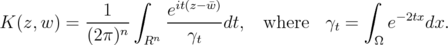 | (1.2) |
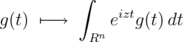
Given a function  on
on  , we shall say that
  reproduces
  if
if
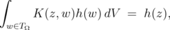 | (1.3) |
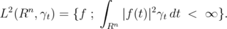
 is the Lebesgue measure on
  . Let
. Let  denote the Bergman space, namely the Hilbert space of all holomorphic functions
  on
on  in which
 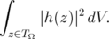 | (1.4) |
The Bergman kernel  is uniquely characterized by the following three properties:
(i) 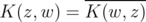 for all
  ;
;
(ii)  reproduces every element in
  in the sense of (1.3);
(iii) 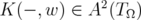 for all
  .
.
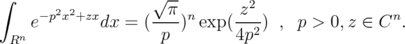
Our formulation of  in (1.2) clearly satisfies condition (i). Therefore, to prove the theorem, we need to check conditions (ii) and (iii). This will be done by Propositions 2.4 and 2.5 in the next section.
2. The Bergman kernel on tube domains
Let  be a bounded strictly convex domain in
  , and let
  be the tube domain as defined in (1.1). Since
  is strictly convex,
  is strictly pseudoconvex.
Let  and
and  be defined as in (1.2). The Bergman space
  consists of holomorphic functions
  which satisfy (1.4). In this section, we show that
  satisfies conditions (ii) and (iii) stated in the Introduction. Let
  denote the polynomial functions, and we define

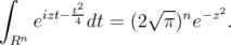
Lemma 2.1  reproduces every element of
  .
.
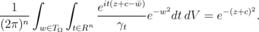
 | (2.1) |
Here  denote the usual dot product. In deriving this identity, we observe that both sides of (2.1) are holomorphic in
  . Therefore, it suffices to check that it holds on the totally real subspace
  . This can be obtained from standard integration tables ([3], 3.323
  2).
2).
Write  on
on  , where
  are variables on
  respectively. Then
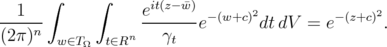
 | (2.2) |
From (2.2), substitute  with
with  , where
  . This gives
Changing the variable  to
to  in LHS gives
Apply  to both sides, we see that
  reproduces the function
  . We carry out the procedure
  for
for  , and Lemma 2.1 follows.
We plan to show that  reproduces every element of
  . In view of Lemma 2.1, this will follow if we can show that
  is a dense subset of the Hilbert space
  . This will be established by the next two lemmas. Our strategy is to convert the problem on
  to another Hilbert space
  by Lemma 2.2, and obtain a result on
  by Lemma 2.3. We then transfer this result back to
  , by Proposition 2.4.
Let  denote the Hilbert space of
  functions on
  , with weight
  given in (1.2). Namely,
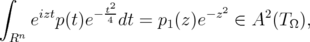
Lemma 2.2 (T. G. Genchev) The transformation
 | (2.3) |
is an isometry from  to
to  , preserving the Hilbert space norms.
 , there exists
  such that
  | (2.4) |
see [1],[2]. This means that the transformation in (2.3) is surjective. In order to see that (2.3) is well-defined, injective and preserves the norms, we shall prove that in (2.4), 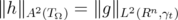 .
.
Write  , and (2.4) gives
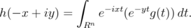
Thus for every fixed  ,
,  is the Fourier transform of
  . By Plancherel's theorem,
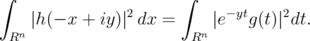
Apply  to both sides, we get
This proves Lemma 2.2. □
Next we define

Lemma 2.3  is dense in the Hilbert space
  .
.
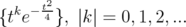 | (2.5) |
is a complete basis of  , and the lemma follows.
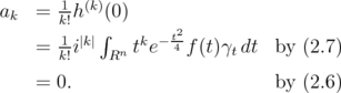
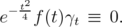
 , and suppose that
  | (2.6) |
for all  . It is easy to see that
  is bounded, so
 . Let
. Let  | (2.7) |
By Lemma 2.2,  . We may assume that
  , and consider the power series expansion
near  . Then
So  vanishes near
  . However, since
  is holomorphic, it follows that
  . By Lemma 2.2,
Since  and
and  are always positive,

This shows that the functions in (2.5) form a complete basis of  , and the lemma is proved. □
We combine Lemmas 2.1, 2.2 and 2.3 to show that:
Proposition 2.4 The function  of (1.2) reproduces every element of
  .
.
Proof: We claim that  is dense in
  . Identity (2.1) implies that
Applying  repeatedly to both sides, we see that if
  is a polynomial, then
for another polynomial  . Namely, the isometry in Lemma 2.2 sends every
to some
By Lemma 2.3,  is dense in
  . Hence
  is dense in
  as claimed.
By Lemma 2.1,  reproduces every element of
  . Therefore, since
  is dense in
  , it follows that
  reproduces every element of
  . □
. □
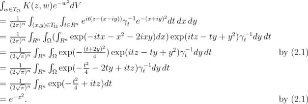
With this result, condition (ii) of  stated in the Introduction is verified. Therefore, to prove the theorem, it remains only to check condition (iii). This is done by the following proposition.
Proposition 2.5 For each fixed 
Proof: Fix  , and consider
  . For any fixed
  , formula (1.2) satisfies

for all  . Further,
  and
and  . Therefore, without loss of generality, we may assume that
 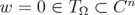 in the statement of this proposition. We want to show that
  . But
. But
and with Lemma 2.2, we get
We have shown that, for each  ,
,  .
.
This result verifies condition (iii) of the Introduction, and the theorem follows.
References
[1] T. G. Genchev, Integral representations for functions holomorphic in tube domains, C. R. Acad. Bulgare Sci. 37 (1984), 717-720. [ Links ]
[2] T. G. Genchev, Paley-Wiener type theorems for functions in Bergman spaces over tube domains, J. Math. Anal. and Appl. 118 (1986), 496-501. [ Links ]
[3] I. S. Gradshteyn, I. M. Ryzhik, Table of Integrals, Series and Products, Academic Press, (1980). [ Links ]
[4] S. Krantz, Function Theory of Several Complex Variables, 2ed. Wadsworth & Brooks/Cole, Pacific Grove 1992. [ Links ]
Ching-I Hsin
Division of Natural Science,
Minghsin University of Science and Technology.
Hsinchu County 304, Taiwan.
hsin@must.edu.tw
Recibido: 6 de mayo de 2004
Aceptado: 28 de marzo de 2005

