Some operator inequalities for unitarily invariant norms^*†

Cristina Cano, Irene Mosconi^‡ and Demetrio Stojanoff^§

^‡ Partially supported by Universidad Nac. del Comahue

^§ Partially supported CONICET (PIP 4463/96), UNLP 11 X350 and ANPCYT (PICT03-09521)

Abstract:
Let be the algebra of bounded operators on a complex separable Hilbert space . Let be a unitarily invariant norm defined on a norm ideal . Given two positive invertible operators and , we show that , . This extends Zhang's inequality for matrices. We prove that this inequality is equivalent to two particular cases of itself, namely and . We also characterize those numbers such that the map given by is invertible, and we estimate the induced norm of acting on the norm ideal . We compute sharp constants for the involved inequalities in several particular cases.

Keywords and phrases: Positive matrices; Inequalities; Unitarily invariant norm.

AMS Subject Classification: Primary 47A30, 47B15.

1. INTRODUCTION

Let be a Hilbert space and denote by the algebra of bounded linear operators on . In 1990, Corach-Porta-Recht [6] show that, for every invertible selfadjoint operator and for every , it holds that

(1)

Several authors have proved generalizations and alternative proofs of inequality (1). For example, Bhatia and Davis [3], Kittaneh (in two different ways, see [11] and [12]), and Andruchow, Corach and Stojanoff [2]. On the other hand, in 1993, Livshits and Ong [14] studied the invertibility of the map for not necessarily selfadjoint . In 2001, Seddik, [15] proved that, for invertible and positive, and ,

(2)

In 1999 Zhan [18] showed that, given two positive invertible matrices , , and , then

(3)

for every unitarily invariant norm on .

In this paper we work with unitarily invariant norms defined in some ideal of (see Remark 2.1 or Simon's book [17]). We show that, for every unitarily invariant norm , the following inequalities are equivalent, for every :

(4)

(5)

(6)

We give a proof of inequality (6), using a technical result about unitarily invariant norms, which allows us to obtain a reduction to the matricial case. In this case, we use a result of Bhatia and Parthasarathy [4], and some properties of the Hadamard product of matrices. This result was previously proved for in [2], for not necessarily positive , and . We study the operators associated to the three mentioned inequalities, and their restriction as operators on the norm ideal . We compute their spectra and, in some cases, their reduced minimum moduli (also called conorms). The rest of the paper deals with the estimation of sharp constants for inequality (5), with respect to the usual norm of . We get the optimal constant, if one restricts to operators . Using the notion of Hadamard index for positive matrices, studied in [7], we compute, for a fixed , the constant

for (see Proposition 5.6). Finally, we give some partial results for , in lower dimensions, showing numerical estimates of sharp constants. For and , we characterize the best intervals such that the inequality (6) holds in for every .

In section 2, we fix several notations and state some preliminary results. We expose with some detail the theory of unitarily invariant norms defined on norm ideals of , proving some technical results in this area. In section 3, we show the equivalence of the mentioned inequalities and we give the proof of (6). In section 4, we study the associated operators. In section 5, we describe the theory of Hadamard index, and we use it to obtain a description of the constant . In section 6 we study the case of matrices of lower dimensions.

We wish to acknowledge Prof. G. Corach who shared with us fruitful discussions concerning these matters.

2. PRELIMINARIES

Let be a separable Hilbert space, and be the algebra of bounded linear operators on . We denote the ideal of compact operators, the group of invertible operators, the set of hermitian operators, the set of positive definite operators, the unitary group, and the set of invertible positive definite operators.

Given an operator , denotes the range of , the nullspace of , the spectrum of , the adjoint of , the modulus of , the spectral radius of , and the spectral norm of . Given a closed subspace of , we denote by the orthogonal projection onto .

When , we shall identify with , with , and we use the following notations: for , for , for , and for . A norm in is called unitarily invariant if for every and .

Remark 2.1. The notion of unitarily invariant norms can be defined also for operators on Hilbert spaces. We give some basic definitions (see Simon's book [17]): Let . Then also . We denote by , the sequence of eigenvalues of , taken in non increasing order and with multiplicity. If , we take for . The numbers are called the singular values of .

Denote by the set of complex sequences which converge to zero. Consider the set of sequences with finite non zero entries. For , denote . A gauge symmetric function (or symmetric norm) is a map which satisfy the following properties:

• is a norm on ,
• for every ,
•and is invariant under permutations. We say that is normalized if . For , define

A unitarily invariant norm in is a map given by , , where is a symmetric norm. The set

is a selfadjoint ideal of , called the norm ideal associated to . Then is a Banach space, and the following properties hold:

1. If , then , and for every .
2. If has finite rank, then , because .
3. If , then .
4. Given and such that then and .
5. For every and , there exists a finite rank operator such that .

Some well known examples of unitarily invariant norms are the Schatten -norms , for , and the Ky-Fan norms , . The usual norm, which coincides with and when restricted to , is also unitarily invariant.

Proposition 2.2. Let be an unitarily invariant norm on an ideal . Let be a increasing net of projections in which converges strongly to the identity (i.e., for every ). Then

Proof. By Remark 2.1, for every , there exists a finite rank operator such that . For every and every projection , it holds that . In particular, for every . Hence, we can assume that . Given , denote . Since and

it suffices to prove that . Fix . Note that . Therefore

This implies that , and all these operators act on the fixed finite dimensional subspace , where the convergence of operators in every norm (included ) is equivalent to the SOT (or strong) convergence.

Remark 2.3. Let be a unitarily invariant norm defined on a norm ideal . The space can be identified with the algebra of block matrices with entries in , denoted by . Denote by the ideal of associated with the same norm (i.e., by using the same symmetric norm ). Then, the following properties hold

1. Let , and define as any of the following matrices
   
   Then , , and if and only if .
2. Under the mentioned identification, .

Given denote by the Hadamard product . Every defines a linear map given by

(7)

Given a norm on , it induces a norm of the linear map by means of

(8)

The following result collects two classical results of Schur about Hadamard (or Schur) products of positive matrices (see [16]), and a generalization of the second one for unitarily invariant norms, proved by Ando in [1, Proposition 7.7] .

Proposition 2.4 (Schur). Let and . Then

1. If then also .
2. Denote by . Then

   (9)

   for every unitarily invariant norm on .

3. EQUIVALENT INEQUALITIES Theorem 3.1. Let and be an unitarily invariant norm on an ideal . Then the following inequalities are equivalent:

1. , for every and .
2. , for every and .
3. , for every and .

Proof. It is clear that 1 implies 2 and 3. Suppose that 2 holds. Consider the space . For and , define the operators

Then

Therefore, as for every , then

This shows . The same arguments using show . □

Remark 3.2. As said in the Introduction, the inequality 2 of Theorem 3.1 was proved, for the usual norm, by Corach-Porta-Recht in [6] with (and not necessarily positive), and by Ameur Seddik in [15] with . The inequality 1 of Theorem 3.1 was proved, in the finite dimensional case, by X. Zhan in [18], for . In the rest of this section, we give a proof of inequality 2 of Theorem 3.1 for in the general setting.

Lemma 3.3. Let , and . Let be given by

Then for every .

Proof. Note that . These numbers are well defined because for every and . Bhatia and Parthasarathy [4] proved that, for and , the matrix with entries

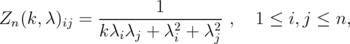(10)

satisfies for every and if and only if

On the other hand, if , then the matrix By Propposition 2.4, for every . □

Theorem 3.4. Let and . Then, for every unitarily invariant norm on an ideal , and for every ,

Proof. We follow the same steps as in [6]. By the spectral theorem, we can suppose that is finite, since can be approximated in norm by operators such that each is finite. We can suppose also that , by choosing an adequate net of finite rank projections which converges strongly to the identity and replacing by . Indeed, the net may be chosen in such a way that and for every . Note that, by Proposition 2.2, converges to for every .

We can suppose that is diagonal by a unitary change of basis in . Take . Then , where

(11)

Since for every , , it follows that, if , then for every . Consider the matrix given by . Hence, in order to prove inequality (6) for every , it suffices to show that for and . By Lemma 3.3, for every . Finally, note that , Therefore, inequality (6) holds by Eq. (9) in Proposition 2.4. □

As a consequence of this result and Theorem 3.1, we get an infinite dimensional version, for every unitarily invariant norm, of Zhang inequality:

Corollary 3.5. Let and . Then, for every unitarily invariant norm on an ideal , and for every ,

Corollary 3.6. Let and . Then, for every unitarily invariant norm on an ideal , and for every ,

4. THE ASSOCIATED OPERATORS

In this section we study the operators associated with the inequalities proved in the previous section. Given and , we consider the bounded operator associated with inequality (4):

(12)

Hence, for every unitarily invariant norm defined on an ideal , inequality (4) means that for , . Given and , define the operators and associated with inequalities (6) and (5): and . In this section we characterize, for fixed , those such that is invertible. In some cases we estimate, for a given norm on some ideal of , the induced norms of their inverses.

Remark 4.1. Let . Denote by the operator given by, . It is clear that . Hence for every norm ideal induced by a unitarily invariant norm . The following properties are easy to see:

1. .
2. The map is sesqui linear.
3. If , then and .

Proposition 4.2. Let . Denote by . Then

Moreover, has the same spectrum, if it is considered as acting on any norm ideal associated with a unitarily invariant norm.

Proof. Fix the norm ideal and consider the restriction . Let be given by , . Note that . Therefore, by the known properties of the Riesz functional calculus for operators on Banach spaces (in this case, the Banach space is and the map is ), it suffices to show that .

Given , denote by (resp. ) the operator given by (resp. ), . By Remark 2.1, these operators are bounded. If , then , and similarly for . Hence and . Note that . Therefore

Given , and , let be unit vectors such that and . Such vectors exist because and are selfadjoint operators. Consider the rank one operator . Then, by Remark 4.1, . Hence

Therefore , because . This shows that , and the proof is complete. □

Corollary 4.3. Let and . Then is invertible if and only if .

Proof. Just note that Id. Then apply Proposition 4.2. □

Remark 4.4. Let be a unitarily invariant norm defined on a norm ideal . By Remark 2.1, for and . Given a linear operator , we denote by the induced norm:

By a standard argument and using the continuity of "taking inverse", one can show that, for fixed, the map is continuous.

Proposition 4.5. Let and . Let be a unitarily invariant norm defined on a norm ideal . Then . Moreover, if , then .

Proof. The inequality follows from Corollary 3.5. Suppose that is an eigenvalue for both and . Let be unit vectors such that and . Consider . Then, since and , it is easy to see that . Hence, in this case. An easy consequence of spectral theory is that every such that can be arbitrarily approximated by positive invertible operators such that is a isolated point of their spectra, hence an eigenvalue. Applying this, jointly for and , for some , and using the fact that the map is continuous, the proof is completed. □

Corollary 4.6. Let and . Let be a unitarily invariant norm defined on a norm ideal . Then . If there exists such that also , then also .

Proof. The first case follows applying Proposition 4.5 with . Note that the hypothesis becomes obvious. For the second, take and . Note that . □

Remark 4.7. The Forbenius norm works on the ideal of Hilbert Schmit operators, which is a Hilbert space with this norm. In this case, the operator defined in Eq. (12) is positive, so that . Therefore, Proposition 4.2 gives the sharp constant for inequality (4) for this norm. Observe that if and only if .

5. SHARP CONSTANTS AND HADAMARD INDEX

Preliminary results. In this subsection, we shall give a brief exposition of the definitions and results of the theory of Hadamard index, which we shall use in the rest of the section. All the results are taken from [7].

Denote by and , the matrix with all its entries equal to . Given and a norm on , we define the -index of by

and the minimal index of by

The index relative to the spectral norm on will be denoted by , and the index relative to the 2-norm tr , , is denoted by .

Proposition 5.1. Let . Then if and only if .

If , then

(13)

Theorem 5.2. Let with nonnegative entries such that all . Then the following conditions are equivalent:

1. There exist with nonnegative entries such that
2. .

Theorem 5.3. Let such that for all . Then there exists a subset of such that . Therefore and

Let , and . We consider

(14)

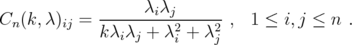
Proposition 5.4. Let , . Consider the matrix defined before. Then if and only . More precisely,

1. If (i.e. #L = 1), then and .
2. If , then the image of is the subspace generated by the vectors and .
3. If , say , denote . Then

   (15)

4. If then , because .

Sharp constants for positive operators. In the rest of this section, we shall use the results above in order to get the sharp constants for inequality (5), if we consider only operators . Remark 5.5. Proposition 5.4 says that, in most cases (i.e. ), . On the other hand, in order to apply index theory for the matrix , we need that . Since if and only if (by the definition of the minimal index), we can only consider the case , in general. In this case, it is easy to check that

(16)

Hence, applying Proposition 5.4, we get formulas for in any case.

We shall compute using Theorem 5.3. Hence, we shall use the principal minors of , which are matrices of the same type. Let , and the induced vectors. Then

Claim: If then, .

Indeed, by Proposition 5.4, , because . Note that every must satisfy , because span . By Proposition 5.4, , where . As all entries of are strictly positive, if and , then . Therefore, the Claim follows from Theorem 5.2.

Hence, if , then . If , let such that . By Theorem 5.2 there exists a vector such that . Let and Easy computations show that, if we denote , then and, by Theorem 5.2, . Moreover, by equations (15) and (16),

Therefore, in order to compute using Theorem 5.3, we have to consider only the diagonal entries of and some of its principal minors of size . If and then, by equations (13) and (16),

Easy computations show that, if , this is equivalent to , which implies that . So, by Theorem 5.3,

(17)

where and

Now we can characterize the sharp constant for inequality (5), if we consider only operators .

Proposition 5.6. Given and , denote by the greatest number such that for every . Then where and

In particular, if , then .

Proof. We shall use the same steps as in the proof of Theorem 3.4 (and [6]). By the spectral theorem, we can suppose that is finite, since can be approximated in norm by operators such that is a finite subset of , for all and is dense in . So (and ) converge to (resp. ).
We can also suppose that , by choosing an adequate net of finite rank projections which converges strongly to the identity and replacing by . Indeed, the net may be chosen in such a way that and for all . Note that for every , converges to .
Finally, we can suppose that is diagonal by a unitary change of basis in . In this case, if are the eigenvalues of (with multiplicity) and , then . Note that all our reductions (unitary equivalences and compressions) preserve the fact that . Now the statement follows from formula (17). If then , since is the infimum of the empty set. Note that is attained at , because the map is decreasing on . □

6. NUMERICAL RESULTS

Let and . Denote by Corollary 3.6 says that, if , then for every . On the other hand, Corollary 4.6 says that, if there exists , then. In this section we search conditions for which assure that. As in the proof of Theorem 3.4, we can assume that for some . In this case, we have that, where is the matrix defined in Eq. (14). Consider the matrix with entries

(18)

. Then, for , . Denote by the map given by , for . We conclude that .

Remark 6.1. There exists an extensive bibliography concerning methods for computing the norm of a Hadamard multiplier like . The oldest result in this direction is Schur Theorem (Proposition 2.4) for the positive case. We have applied this result in the proof of Theorem 3.4, but it is not useful in this case, because . The most general result is 1983's Haagerup theorem [10], which gives a complete characterization, but it is not effective. There exist also several fast algorithms (see, for example, [9]) which allow to make numerical experimentation for this problem. For example, we have observed that the behavior of the map , for any fixed , is chaotic. But, as a great number of examples suggest, it seems that if and only if . Note that these cases are exactly those considered in Corollary 4.6.

Cowen and others [8] and [9] proved the following result for hermitian matrices:

Theorem 6.2. Let such that . Suppose that has rank two, or that has one positive eigenvalue and non positive eigenvalues. Then the following conditions are equivalent:

1. .
2. If and , then .
3. For , it holds that .

Suppose that satisfies or Since that map is increasing on and it is decreasing on , it follows that the matrix of Eq. (18) satisfies . This suggests that we could apply Theorem 6.2 for our problem. Unfortunately, for , has rank greater than two, and it can have more that one positive eigenvalue. We prove the following result:

Proposition 6.3. Let . Suppose that , or S. Then

Proof. Suppose that with or . Let as in equation (18), for . Then . Hence, since , can apply Theorem 6.2. Then, in order to prove that , it suffices to verify the inequality Note that

Straightforward computations with show that , since the polynomial in this case. A similar analysis shows that still for . The result follows by applying Theorem 6.2. □

It was proved by Kwong (see [13]) that, if , then the matrix defined in Eq. (10), is positive semidefinite in the following cases: and , and , and and . Therefore, by the proof of Theorem 3.4, inequality (6) holds in in these cases, for every unitarily invariant norm. Note that the proof Theorem 3.1 does not give similar estimates for the inequalities (4) and (5), because one needs to duplicate dimensions.

A numerical approach suggests that these intervals are optimal, both for the positivity of the matrix , defined in Eq. (11), and for inequality (6). In the case of , if and then, using symbolic computation with the software Mathematica, one obtains a kind of "proof" of the fact that for every if and only if The principal sub matrices of have the form , and they live in for every . Therefore,

Likewise, for the matrix case, it suffices to study , for , and one obtains similar results.

Denote by the maximum number such that inequality (6) holds in for the spectral norm. By the preceding comments, and the proof of Theorem 3.4,

Computer experimentation using the softwares Mathematica and Matlab suggests that, also in this case, , , and , for . In other words, inequality (6) holds for in the same intervals as it holds that for every .

References

[1]    T. Ando, Majorization and inequalities in matrix theory, Linear Algebra Appl. 199: 17-67, 1994.         [ Links ]

[2]    E. Andruchow, G. Corach and D. Stojanoff, Geometric operator inequalities, Linear Algebra Appl. 258: 295-310, 1997.         [ Links ]

[3]    R. Bhatia, and CH. Davis, More matrix forms of the Arithmetic-Geometric mean inequality, SIAM J. Matrix Anal. Appl. 14: 132-136, 1993.         [ Links ]

[4]    R. Bhatia and K. R. Parthasarathy, Positive definite functions and operator inequalities, Bull. London Math. Soc. 32: 214-228, 2000.         [ Links ]

[5]    R. Bhatia, Matrix Analysis, Springer-Verlag, New York, 1997.         [ Links ]

[6]    G. Corach, H. Porta and L. Recht, An operator inequality, Linear Algebra Appl. 142: 153-158, 1990.         [ Links ]

[7]    G. Corach and D. Stojanoff, Index of Hadamard multiplication by positive matrices II, Linear Algebra Appl. 332-334 (2001), 503-517.         [ Links ]

[8]    C. C. Cowen, K. E. Debro and P. D. Sepansky, Geometry and the norms of Hadamard multipliers, Linear Algebra Appl. 218: 239-249, 1995.         [ Links ]

[9]    C. C. Cowen, P. A. Ferguson, D. K. Jackman, E. A. Sexauer, C. Vogt y H. J. Woolf, Finding Norms of hadamard multipliers, Linear Algebra Appl. 247, 217-235 (1996).         [ Links ]

[10]    U. Haagerup, Decompositions of completely bounded maps on operator algebras, unpublished manuscript.         [ Links ]

[11]    F. Kittaneh, A note on the arithmetic-geometric inequality for matrices, Linear Algebra Appl. 171 (1992), 1-8.         [ Links ]

[12]    F. Kittaneh, On some operator inequalities, Linear Algebra Appl. 208/209:19-28, 1994.         [ Links ]

[13]    M.K. Kwong, On the definiteness of the solutions of certain matrix equations, Linear Algebra Appl. 108: 177-197, 1988.         [ Links ]

[14]    L. Livshits and S. C. Ong, On the invertibility properties of the map and operator-norm inequalities, Linear Algebra Appl. 183: 117-129, 1993.         [ Links ]

[15]    A. Seddik, Some results related to the Corach-Porta-Recht inequality, Proceedings of the American Mathematical Society, 129: 3009-3015, 2001.         [ Links ]

[16]    I. Schur, Bemerkungen zur theorie de beschränkten bilineareformen mit unendlich vielen veränderlichen, J. Reine Angew. Math. 140: 1-28, 1911.         [ Links ]

[17]    B. Simon, Trace ideals and their applications, London Mathematical Society Lecture Note Series, 35, Cambridge University Press, Cambridge-New York, 1979.         [ Links ]

[18]    X. Zhan, Inequalities for unitarily invariant norms, SIAM J. Matrix Anal. Appl. 20:466-470, 1999.         [ Links ]

Cristina Cano
Depto. de Matemática,
FaEA-UNC,
Neuquén, Argentina.
cbcano@uncoma.edu.ar

Irene Mosconi
Depto. de Matemática,
FaEA-UNC,
Neuquén, Argentina.
imosconi@uncoma.edu.ar

Demetrio Stojanoff
Depto. de Matemática,
FCE-UNLP, La Plata, Argentina
and IAM-CONICET.
demetrio@mate.unlp.edu.ar

Recibido: 3 de junio de 2005
Aceptado: 21 de noviembre de 2005