


Services on Demand
Journal

Article
 English (pdf)
 Article in xml format
 Article references
 Send this article by e-mail
Indicators
-
 Cited by SciELO
Related links
-
 Similars in
SciELO
Similars in
SciELO
Share

 Permalink
Revista de la Unión Matemática Argentina
Print version ISSN 0041-6932On-line version ISSN 1669-9637
Rev. Unión Mat. Argent. vol.46 no.2 Bahía Blanca July/Dec. 2005
Recent progress in the well-posedness of the Benjamin-Ono equation
Carlos E. Kenig *
Dedicado a la memoria de Pucho Larotonda
* Supported in part by NSF
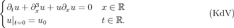
In this note, I will describe some recent progress on the well-posedness theory of the Benjamin-Ono (BO) equation, one of the challenging, well-studied, but not completely understood, dispersive models in one space dimension. To put matters in perspective, I will start by describing the theory for the Korteweg-de Vries (KdV) equation, another well-studied dispersive model, for which the well-posedness theory has been well-understood for some time. (For references for the results described here see [Bou93], [KPV93], [KPV96], [CCT03], [CKS+03], [BP], [IK] and the references in those papers.) Both equations are completely integrable and possess infinitely many conserved quantities (for real-valued solutions, to which we will stick to from now on). Recall that
By local in time well-posedness (l.w.p.), with data  in a Banach space of data
  , we will mean existence, uniqueness, persistence in
  and continuous dependence of the flow on the data in
  , for a time
  (
(![u0 ∈ B → u ∈ C([ - T,T ];B)](/img/revistas/ruma/v46n2/2a067x.png) is continuous). If
is continuous). If 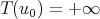 , we have global in time well-posedness (g.w.p.). Note that KdV is time reversible (
 a solution
 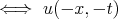 is a solution) which explains the symmetric time intervals. The data space
  will usually be taken as the Sobolev space
  , where
  and
and  . When
  ,
,  consists of
  such that
  . An important difficulty in establishing l.w.p. for KdV in
  is the presence of the derivative in the non-linear term
  which needs to be "absorbed". In the late 70s it was observed that the energy method (a method used for the study of symmetric hyperbolic systems) applies to give l.w.p. for KdV in
  , for suitable
  (Bona-Smith). Here, the energy method only uses the antisymmetry of
  , which gives
  . It hinges on having a priori control of
  in terms of
  . For instance, when
  ,
,  , Sobolev embedding gives
 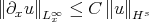 and this control is immediate. Thus (Bona-Smith) we obtain l.w.p. in
  ,
,  . Note however that the same argument applies to Burger's equation
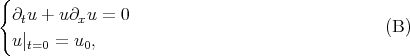
giving l.w.p. in  ,
,  . But, for (B), this is the sharp index for l.w.p. and people became interested in whether this result can be improved or not for KdV. It is instructive to consider conserved quantities for KdV:
  ,
,  are constant in time. The second one is the Hamiltonian associated to KdV. Note that they imply the a priori bounds
 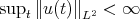 , and
, and 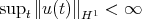 . They do not give control on
 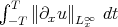 , so that the energy method cannot be applied. (Uniqueness is in question.) Nevertheless, in 1983, Kato and, independently, Kruzhkov-Faminski obtained the 'a priori' estimates (local smoothing)
which, combined with the previous a priori bounds, led to the existence of 'weak solutions' with data in  ,
,  . Their uniqueness could not be established.
In the late 80s and early 90s, Kenig-Ponce-Vega introduced into the problem methods of harmonic analysis and were able to make further progress. They proved (91) that KdV is l.w.p. in  ,
,  and g.w.p. in
  . The second result is a direct consequence of the first one and the Hamiltonian. Two proofs were given. The first one established control of
  , without using Sobolev (an "enhanced energy method"). The second one used an integral equation which could be solved by Picard iteration using the contraction mapping principle in a suitable Banach space of solution functions
  . The proofs relied on the same estimates. I will now briefly describe the second proof.
Consider the associated linear problem
whose solution is  , where the homogeneous solution operator is
 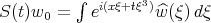 (Duhamel's principle, method of variation of the constants). We let
  , and thus we need to solve the integral equation
  . Let
. Let  , the 'dispersive' character of the equation is reflected on the lower bound for
  . In order to apply the contraction principle in a suitable space
  , we exploited the lower bound of
  be establishing the sharp local smoothing estimate
In order to estimate the nonlinear term  , we paired this with the maximal function estimate
which is close to the restriction problem in harmonic analysis and which uses the curvature of the level sets of  .
.
Further progress was made by Bourgain (93) who introduced new function spaces in which to do the contraction, establishing l.w.p. and g.w.p. in  . The first (simple but important) observation of Bourgain's is that to prove l.w.p. for
  one can replace the above integral equation with

 ,
,  for
for  . From now on
  will denote the Fourier transform of 1 or 2 variables and
  its inverse. It is easy to see that
  . Also, it is not difficult to see that
In order to solve (+) by the contraction map principle in a solution space  , for data which are (small) in
  and obtain our l.w.p. result, one needs:
 ,
, 
 .
. Bourgain introduced the spaces ( )
)

It is easy to see that for  ,
,  ,
,  , and that for
 . All boils down then to the "bilinear smooting" estimate
which Bourgain showed to hold for some  .
.
Note that
The key ingredient in the proof of the "bilinear smoothing" estimate is: let

With  (
( ), this is used in conjunction with:

to use our information on  , to 'trade' (
 ) for
) for  , in order to "absorb the
  -derivative". Lower bounds on
  are crucial for this.
Bourgain's method was extended to  ,
,  by Kenig-Ponce-Vega (96), to obtain l.w.p.
A difference to point out between obtaining w.p. using the energy method (possibly "enhanced") and the contraction principle is that, in the first case one only obtains the continuity of the solution map  , while in the second case (for analytic nonlinearities) one obtains that
  is real analytic.
Christ-Colliander-Tao (2003) showed that, for KdV, for  , the solution map is not uniformly continuous on bounded sets, so that the KPV result is in a sense optimal. Moreover, by developing a new general method (the method of almost conservation laws) Colliander-Keel-Staffilani-Takaoka-Tao (2001) were able to show g.w.p. for KdV,
  .
.
The ideas and techniques explained have had a multitude of other applications, to, for example, non-linear Schrödinger and non-linear wave equations, and to many other problems, not only dealing with well-posedness issues.
I will now turn to the (BO) equation:
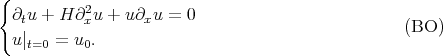
Here  denotes the Hilbert transform on
  defined by
 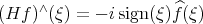 . Thus, we have a non-local operator. As I mentioned before, this is a model in water wave theory which like KdV is completely integrable and has infinitely many conserved quantities. My interest in it comes from the fact that there is an exact balance between the strength of the nonlinearity and the smoothing properties of the linear part, which prevents the direct application of the techniques we discussed before. Notice first that
  is antisymmetric, while
  is symmetric, so that
 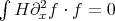 . Thus, the energy method applies and shows that (BO) is l.w.p. in
  ,
,  (Iorio 86). The first two conserved quantities for (BO) are
  and the Hamiltonian
  . It has infinitely many such conserved quantities, each corresponding to a derivative of order
  ,
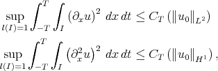
,  . (The next ones correspond to 1 and 3/2 derivatives.) In 91 Ponce used a version for (BO) of Kato's smoothing effect to show that for data
  in
in  one can control
  , to get by an "enhanced" energy method l.w.p. in
  and hence
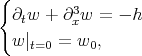
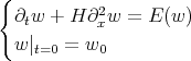
  by the conservation law. The associated linear problem is
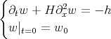
whose solution is

 . Thus,
  . This means that in the "local smoothing" estimate, we only gain 1/2 derivative, instead of 1:
Thus, we cannot 'absorb' the full derivative in the non-linearity  and the KPV argument using local smoothing and maximal function estimates does not apply. In 93, in connection with work on non-linear Schrödinger equations with derivatives in the non-linearity, Kenig-Ponce-Vega discovered the following inhomogeneous "double smoothing" estimate: for
  ,
,

One can then show ([KPV93]) that (BO) is l.w.p. in  , for data of small norm, by contraction.
How about using Bourgain spaces, for the usual Sobolev spaces? As before, the crucial quantity is  , where now
  . Once can then see that

Note that if  ,
,  ,
,  , but
, but 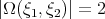 . This is responsible for the fact that for a "bilinear smoothing" estimate of the type
to hold, for any  , we must have
  . Thus, we can only smooth 1/2 a derivative in the "bilinear smoothing" estimate. It turns out that things go catastrophically wrong, as was shown by Molinet-Sant-Tzvetkov (2001): for no
  ,
,  , is the map
 ![Hs( ℝ) ∋ u0 ↦→ u ∈ C([- T, T];Hs( ℝ))](/img/revistas/ruma/v46n2/2a06141x.png) of class
of class  at
at  . Thus, we cannot show l.w.p., for any
  , by contraction, and the mapping
  ,
,  is continuous but not
  . This was strengthened by Koch-Tzvetkov (2003) who showed (for
  ) that his map is not uniformly continuous at
  . These examples exhibit the fact that the interaction of the small frequencies (
 ) with the large frequencies (
 ) are responsible for this catastrophic failure. After this there were 2 results on further "enhancements" of the energy method. Koch-Tzvetkov (2003) showed l.w.p. in
  ,
,  , and then Kenig-Koenig (2003) combined their argument with the 'local-smoothing estimate' of Ponce's to obtain
  .
.
Then, in 2004, there was a breakthrough by Tao, who introduced a "gauge transformation" and used it to prove, by an "enhanced energy method", l.w.p. in  . Because of the higher conservation law, this also shows g.w.p. in
  .
.
Finally, in 2005, Burq-Planchon used Tao's gauge transformation and Bourgain spaces to prove l.w.p. in  ,
,  and hence, by the use of the Hamiltonian, g.w.p. in
  ,
,  . Independently, also in 2005, Ionescu-Kenig showed g.w.p. in
  ,
,  . The rest of the lecture will be devoted to a sketch of some of the ideas in the Ionescu-Kenig proof. Besides the obstacle coming from the "low-high" frequency interaction (Molinet-Saut-Tzvetkov example), if we consider a "bilinear smoothing" estimate for function in Bourgain spaces, with no small frequencies, i.e.:
for functions with  for
for  , one can see that even for functions of "low modulation" (i.e.
  ,
,  ), we must have
  , and even then, there is a "logarithmic divergence" for any
  . This is another difficulty that we need to keep in mind. Our proof proceeds in the following steps:
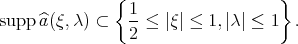
Step 1: We construct a space of data,  , which coincides with
  for frequencies
  ,
,  , and for which, in the small frequencies
  , we have "special structure". (This is reminiscent of the spaces considered by KPV in 93.) One then modifies the Bourgain spaces, for low modulation functions, by adding to it the space of functions
  such that
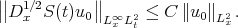
 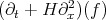 has finite (normalized)
  norm (in physical space). (This norm comes from the "double smoothing" effect mentioned before.) This is inspired by Tataru's work (1998) on wave maps, where the physical space norm is the energy norm. Using these spaces, the "logarithmic divergence" is removed, for functions having "special structure" in the low frequencies, and we show l.w.p. in
  (small norm) by contraction mapping.
Step 2: "Removal of low frequencies": The first point is that for general data  , its low frequency part
  is very smooth and hence by the early results we obtain a global smooth solution
  , with
  as initial data. We then let
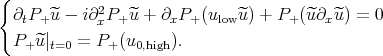
  and write the equation for
  :
:

where  is the high frequency part of
  . The difficulty now comes from the linear term
  which still contains the dangerous "low-high" interactions. To eliminate it, we do a "gauge transformation". Let
  the Fourier multiplier
  . Then
  , so that applying
  to the equation for
  gives
gives
Now, one introduces an "integrating factor", by writing 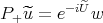 , where
  , which "eliminates" the term
  . This is the "gauge transformation". Note that
  is real-valued, since
  is so, and hence
  is bounded and smooth. We eventually obatin a (system) of equations for
  , of the form
where  . The non-linearity
  is "essentially" of the form
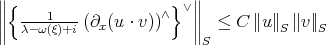
  . We would be in good shape if
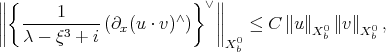
  was a good multiplier of the solution spaces of Step 1. Thus, let
  , say, i.e.,
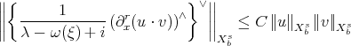
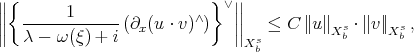
where 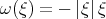 . Let
. Let  be very smooth, say
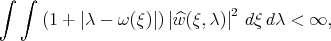
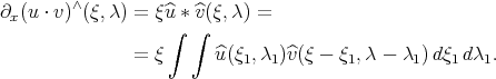
Does  ? Now,
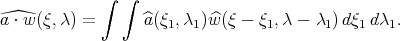
Recall that ![λ - ω( ξ) = [λ1 - ω( ξ1)] + [(λ - λ1) - ω( ξ - ξ1)] + [ω( ξ1) + ω(ξ - ξ1) - ω(ξ)] = Ω(ξ1,ξ - ξ1)](/img/revistas/ruma/v46n2/2a06214x.png) and that, in our situation,
and that, in our situation,  . Thus, if
  , there is a huge change in modulation from the modulation of
  and nothing good can be said. However, for the "high modulation" part of
  , we are fine. Thus, if we write
  ,
,  , we can say nothing about
  , but
, but  . But
. But  . The last term seems troublesome, but we are saved because
  , and the proof proceeds.
[Bou93] J. Bourgain, Fourier transform restriction phenomena for certain lattice subsets and applications to nonlinear evolution equations. II. The KdV-equation, Geom. Funct. Anal. 3 (1993), no. 3, 209-262.
[BP] N. Burg and F. Plauchon, On well-posedness for the benjamin-ono equation, preprint, http://arxiv.org/abs/math.AP/0509096, v1, September 5, 2005, revised v2, November 25, 2005.
[CCT03] Michael Christ, James Colliander, and Terrence Tao, Asymptotics, frequency modulation, and low regularity ill-posedness for canonical defocusing equations, Amer. J. Math. 125 (2003), no. 6, 1235-1293.
[CKS+03] J. Colliander, M. Keel, G. Staffilani, H. Takaoka, and T. Tao, Sharp global well-posedness for KdV and modified KdV on  and
and  , J. Amer. Math. Soc. 16 (2003), no. 3, 705-749 (electronic).
[IK] A. Ionescu and C. Kenig, Global well-posedness of the benjamin-ono equation in low regularity spaces, preprint, http://arxiv.org/abs/math.AP/0508632, August 31, 2005.
[KPV93] Carlos E. Kenig, Gustavo Ponce, and Luis Vega, Well-posedness and scattering results for the generalized Korteweg-de Vries equation via the contraction principle, Comm. Pure Appl. Math. 46 (1993), no. 4, 527-620.
[KPV96] Carlos E. Kenig, Gustavo Ponce, and Luis Vega , A bilinear estimate with applications to the KdV equation, J. Amer. Math. Soc. 9 (1996), no. 2, 573-603.
Carlos E. Kenig
Department of Mathematics,
University of Chicago,
Chicago, IL 60637, USA
Recibido: 23 de marzo de 2006
Aceptado: 7 de agosto de 2006

