Infinitely many minimal curves joining arbitrarily close points in a homogeneous space of the unitary group of a C*-algebra

Esteban Andruchow, Luis E. Mata-Lorenzo, Lázaro Recht, Alberto Mendoza and Alejandro Varela

Dedicated to the memory of Ángel Rafael Larotonda (Pucho).

 

Abstract: We give an example of a homogeneous space of the unitary group of a C*-algebra which presents a remarkable phenomenon, in its natural Finsler metric there are infinitely many minimal curves joining arbitrarily close points.

1. Introduction

In this paper, we give an example of a homogeneous space of the unitary group of a C-algebra which presents a remarkable phenomenon. Namely, in its natural Finsler metric there are infinitely many minimal curves joining arbitrarily close points. More precisely the homogeneous space will be called . The unitary group  of a C-algebra  acts transitively on the left on . The action is denoted by , for and . The isotropy will be the unitary group of a -subalgebra . The Finsler norm in  is naturally defined by , for where projects to in the quotient which is identified to the tangent space . These definitions and notation are borrowed from [1].

This work is part of a forthcoming paper by the same authors which will contain additional results about minimal vectors. We call an element minimal vector if

2. The Minimality Theorem

In [1] the following theorem is proven.

Theorem 2.1. Let be a homogeneous space of the unitary group of a C-algebra . Consider and . Suppose that there exists which is a minimal vector i.e. . Then the oneparameter curve given by has minimal length in the class of all curves in joining to for each with .

We will use the following notation. Let be a unital C-algebra, and a C-subalgebra. Denote and (resp. and ) the sets of selfadjoint (resp. anti-hermitian) elements of and . Let be a Hilbert space, the algebra of bounded operators acting on , and the group of invertible operators.

We call an element a minimal vector if

Note that since for any operator, , it follows that is minimal if and only if

In view of the purpose of this paper stated in the introduction and the previous theorem, to look for minimal curves we have to find minimal vectors and therefore the following theorem is relevant.

Theorem 2.2. An element is minimal if and only if there exists a representation of in a Hilbert space and a unit vector such that

1. .
2. for all .

Proof. The if part is trivial. Suppose that there exist as above. Then if ,

Suppose now that is minimal. Denote by the closed (real) linear span of and the operators of the form for all possible . Note that is positive and is selfadjoint, i.e. .

Denote by the cone of positive and invertible elements of . We claim that the minimality condition implies that . Indeed, otherwise, since is open, there would exist and such that

We may suppose that , so that dividing by we get that for given , ,

(2.1)

Also note that , then for ,

Or equivalently, dividing by ,

In other words, one can find with arbitrarily small norm such that inequality 2.1 holds.

This inequality clearly implies that

On the other hand, since can be chosen with arbitrarily small norm, and is non positive, it is clear that one can choose in order that . Therefore there exists such that . Let us show that this contradicts the minimality of , and thus proves our claim. Indeed, this is stated in lemma 5.3 of [1]:

Lemma 2.3. If for all , then also .

We include its proof. Consider for , . Note that . Otherwise and then the convex combination has norm strictly smaller than for . Note that

That is , which contradicts the hypothesis, and the lemma is proven, as well as our claim.

We have that , with a closed (real) linear submanifold of and open and convex in . By the Hahn-Banach theorem, there exists a bounded linear functional in such that

The functional has a unique selfadjoint extension to , let be the normalization of this functional. Then clearly is a state which vanishes on . Let be the GNS triple associated to this state. Note that since , , and therefore, by the equality part in the Cauchy-Schwartz inequality, it follows that

Moreover, . Since is selfadjoint, this means for all . Putting in the place of , one has that in fact for all . Then,

which concludes the proof.

3. Infinitely many minimal curves joining arbitrarily close points

In this example the homogeneous space is the flag manifold of 4-tuples of mutually orthogonal lines in (1-dimensional complex subspaces). The group of unitary operators in acts on the left in by sending each complex line to its image by the unitary operator (thus preserving the orthogonality of the new 4-tuple complex lines). Consider the canonical flag where is the complex line spanned by the canonical vector in . The isotropy of the canonical flag is the subgroup of 'diagonal' unitary operators.

We consider now the submanifold of  given by

Notice that where is the flag manifold of couples of mutually orthogonal 1-dimensional complex lines in . Notice also that an ordered pair of mutually orthogonal 1-dimensional complex lines in is totally determined by the first complex line of the pair, hence . Furthermore , the Riemann Sphere, hence =.

The minimal curves presented in this example shall be constructed in . For a better geometrical view of those curves we shall identify , via stereographic projection, with the unit sphere  in , hence we shall make the identification .

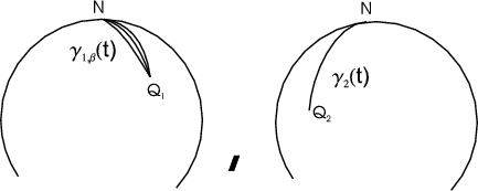
3.1. A description of the minimal curves. Let be the point whose coordinates are both the North Pole, . Let 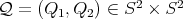be any point of  such that has higher latitude than in  ( is closer to than ).

We will fix so that is above the equator line (and is even higher) and present a family of minimal curves , all joining to . The curve in  will trace the smaller arc of the great circle that contains and . The family of curves will vary continuously with the parameter . Each of the curves of the family will parametrize the smaller arc of some circle in  that joins to ; the arcs will not be great circles but for .

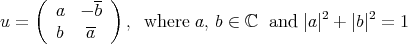
3.2. A precise description of the minimal curves. To present the curves drawn above we give a more manageable description of . We consider the unitary subgroup of the -algebra  of complex matrices, and denote with the subalgebra of diagonal matrices in . The homogeneous space is given by the quotient , where is the subgroup of the diagonal unitary matrices. The group acts on (on the left). The tangent space at 1 (the identity class) is the subspace of anti-hermitian matrices in  with zeroes on the diagonal.

We construct as follows. First consider the subgroup of special unitary matrices build with two, , blocks on the diagonal. We set as the quotient of 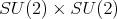by the subgroup of diagonal special unitary matrices. This submanifold is in itself a product of two copies of the quotient of by the subgroup of diagonal matrices in . For the relations among the different groups here mentioned we suggest [2]. We write 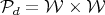and a point of  is a class (in a quotient) which in itself has two components which are also classes. We shall use the notation .

The minimal curves starting at are of the form where the matrices are anti-hermitian matrices with zero trace in  built with two blocks of anti-hermitian matrices on the diagonal (each one with zero trace).

The minimality of the curves is granted by 2.1 for the matrices shall be minimal vectors according to theorem 2.2. In fact, we shall consider of the form

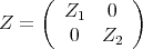
where and are anti-hermitian matrices of the form

(3.2) (3.3)

where , and .

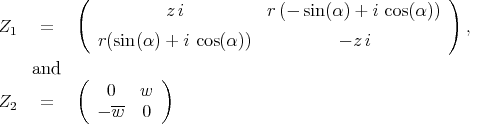
The minimality of these matrices is assured in the case where 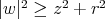. In such case, and, in relation to theorem 2.2, just consider the operator representation of the -algebra  on , together with the unit vector .

3.2.1. The two components of the curves in . The curve in  has two components (in ).

We shall regard the Riemann Sphere  as the complex plane with the point "" added. Consider a matrix in

We consider the mapping from to  is given by

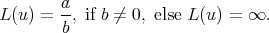
It is clear that this mapping induces an explicit diffeomorphism from the quotient of by its diagonal matrices to the Riemann Sphere .

Consider the unit sphere  in , and let the equatorial plane, , represent the "finite" part of the Riemann Sphere . We set to be the stereographic projection given as by:

Notice that in the class , if , then . If , then , hence , then .

Via a composition of two maps, we define the diffeomorphism  from onto : for we set,

Considering the curve in with as in (3.2) above, and setting , it can be verified that is given by,

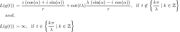
(3.4) (3.5)

Notice then that parametrizes a straight line in . Hence the curve

is an arc of a circle in  (not necessarily a great circle) contained in the plane in that contains both the line , in the equatorial plane, and the North Pole , in . It can be verified that this plane has unit normal vectors given by:

where .

3.2.2. Some observations on the curves and in . Let , where , and let

• In the constructions above, the curve runs over a great circle in  if and only if (equivalently ).
• The curve runs over a great circle in  ( has parameter ).
• The curve varies continuously with the parameter .
• The curve starts at and returns to that point exactly for .
• The curve has constant speed in .
• The curve has constant speed in .

3.2.3. The curves in . Lets give explicit values of the "parameters" and that define and (according to formulas (3.2) and (3.3)), so that for , the curves and join the point to and respectively.

Suppose that the distances from to and in  are and respectively (with ).

By means of some rotation of the sphere  we may suppose that is in the plane generated by and , as in figure 1 below, and we have, .

 

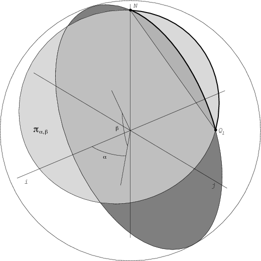
Figure 1: We suppose that is in the plane generated by and

 

For we set so that .

We have to choose the values and that define . This is equivalent to chose via the change of variables given by the equations

The parameters and are shown in figure 1, with the only restriction that the vector

is orthogonal to a plane that contains and .

The parameter is determined after choosing and so that the short arc joining and , in the intersection of the plane with the sphere as in figure 1, has length equal to , from where the value of is drawn.

References

[1]    Durán, C. E., Mata-Lorenzo, L. E. and Recht, L., Metric geometry in homogeneous spaces of the unitary group of a C-algebra: Part I-minimal curves, Adv. Math. 184 No. 2 (2004), 342-366.         [ Links ]

[2]    Whittaker, E. T. "A Treatise on the Analytical Dynamics of Particles and Rigid Bodies", Cambridge University Press, London 1988.         [ Links ]

Esteban Andruchow
Instituto de Ciencias,
Universidad Nacional de Gral. Sarmiento,
J. M. Gutierrez (1613) Los Polvorines, Argentina
eandruch@ungs.edu.ar

Luis E. Mata-Lorenzo
Universidad Simón Bolívar, Apartado 89000,
Caracas 1080A, Venezuela
lmata@usb.ve

Lázaro Recht
Universidad Simón Bolívar, Apartado 89000,
Caracas 1080A, Venezuela, and
Instituto Argentino de Matemática, CONICET, Argentina
recht@usb.ve

Alberto Mendoza
Universidad Simón Bolívar, Apartado 89000,
Caracas 1080A, Venezuela
jacob@usb.ve

Alejandro Varela
Instituto de Ciencias,
Universidad Nacional de Gral. Sarmiento,
J. M. Gutierrez (1613) Los Polvorines, Argentina
avarela@ungs.edu.ar

Recibido: 23 de marzo de 2006
Aceptado: 7 de agosto de 2006