


Services on Demand
Journal

Article
 English (pdf)
 Article in xml format
 Article references
 Send this article by e-mail
Indicators
-
 Cited by SciELO
Related links
-
 Similars in
SciELO
Similars in
SciELO
Share

 Permalink
Revista de la Unión Matemática Argentina
Print version ISSN 0041-6932On-line version ISSN 1669-9637
Rev. Unión Mat. Argent. vol.47 no.1 Bahía Blanca Jan./June 2006
Integrability of f-structures on generalized flag manifolds
Sofía Pinzón
Financiado parcialmente por COLCIENCIAS, contract No. 138-2004.
Abstract: Here we consider a generalized flag manifold  and a differential structure
  which satisfy
  these structures are called f-structures. Such structure
  determines in the tangent bundle of
  some
some  invariant distributions. Since flag manifolds are homogeneous reductive spaces, they certainly have combinatorial properties that allow us to make some easy calculations about integrability conditions for
  itself and the distributions that it determines on
  An special case corresponds to the case
  , the unitary group, this is the geometrical classical flag manifold and in fact tools coming from graph theory are very useful.
A tensor field  of type (1,1) on a Riemannian manifold is called an
  -structure if
  , and almost complex if
  Obviously, an almost complex structure is also an
  -structure. Integrability of almost complex structures is equivalent to the associate Nijenhuis tensor being null. In [7] Ishihara and Yano present an analogous theorem in the case of
  -structures. We use their results to study integrability conditions when one generalized flags manifold are consider.
Let  be a semisimple Lie group. A generalized flag manifold with Lie group
  is a reductive homogeneous space
  where
where  is a centralizer of a torus. This manifold can be expressed as a
  where
where  is the compact connected form of
  and
and  This manifold and its tangent space
  have a characterization in terms of the corresponding root system terms. We will consider along this paper a generalized flag manifold together with an invariant metric
  and an
  -invariant
  -structure
  meaning that
  commute with the adjoint action of
  Ww will denote by
  the complexification of this
  -structure, which is diagonalizable with eigenvalues
  and eigenspaces
  In analogy with the almost complex case we will distinguish between vectors of types
  ,
,  or
or  corresponding to the eigenvalues of
  respectively.
The integrability of  the distributions that it determines in
  and the properties of that distributions are our central topic. We characterize in root terms and in graph theoretical terms the integrability conditions.
In particular, we get that the only integrable  -structure, different from the null structure, in the maximal classical flag manifold is the structure which corresponds to the integrable almost complex structure, that is, in graph theoretic terms which corresponds to the canonical tournament.
Theorem A necessary and sufficient condition for  to be integrable is that
  Therefore
  is integrable if in
  there are not exist triples of type
  or
or  In
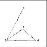
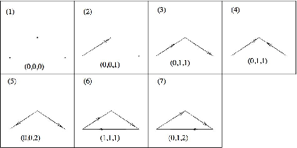
In  this condition is equivalent to the associated digraph avoiding the subdigraphs (2), (3), (4), (5) or (6) in figure 2, that is, the digraph associated to
  must be isomorphic to the null digraph or the canonical tournament.
The Theorem above will appear like Theorem 8.8 and with this result we generalized a Theorem from Burstall [4] given in the context of almost complex structures where he shows that one almost complex structure is integrable if and only if its associated tournament is isomorphic to the canonical tournament, that is, the tournament which does not have three-cycles in root terms it avoids {0,3,0}-triples.
In this section we shall briefly review some general concepts involving generalized flag manifold and some operators and structures which we will use in all this paper. First we need to present a survey about some operators in differential geometry, then we will calculate them specifically on generalized flag manifolds, to this topic we used, specially Props I.3.2, I.3.4, I.3.5 in [8].
2.1. Operators on a general differential manifold.
- Lie derivative. This is the resulting derivative when a tensor field or a differential form is differentiated with respect to a vector field.
1) Lie derivative on tensor fields:![LieX Y = [X, Y]](/img/revistas/ruma/v47n1/1a1051x.png) .
.
2) Lie derivative on tensors: On tensors of type (1,r) we get
 ![∑r (LieX K)(Y1, ...,Yr) = [X, K(Y1, ...,Yr)] - K(Y1, ...,[X, Yi]...,Yr). i=1](/img/revistas/ruma/v47n1/1a1053x.png)
(1) 3) Lie derivative on forms: If
 is an
is an  -form, then
![r ∑ (LieXω)(Y1, ...,Yr) = X ω(Y1, ...,Yr) - w(Y1, ...,[X, Yi]...,Yr). i=1](/img/revistas/ruma/v47n1/1a1056x.png)
(2) - The riemannian invariant connection. Each Riemannian manifold admits a unique metric connection with vanishing torsion, called the Riemannian connection or Levi-Civita connection, and it satisfies
![T(X, Y ) = [X, Y ] - ∇X Y + ∇Y X = 0](/img/revistas/ruma/v47n1/1a1058x.png) and
and  where
where  is the metric on the manifold and
  is the torsion tensor [8].
1) The covariant derivative on tensors. Given a tensor field
 of type
  the covariant differential
  of
of  is a tensor field of type
  defined as follows.
2) The covariant derivative on forms. If
 is an
is an  -form, then
- Exterior derivative on forms. Exterior differentiation
 can be characterize as follow:
  is a degree-increasing
  -linear mapping, that is if
  is a
is a  form,
form,  is a
is a  -form;
- signed derivation w.r.t. the wedge product, that is, if
 is a
is a  -form and
  is a
is a  -form, then
  ;
; 
- For 0-forms
 is defined by
 extends to
  -forms coefficient-wise, using basis expansions, resulting in
Here
 means that you not consider that component. On functions the 1-form
  is defined by
  Otherwise we get
(3) On 1-forms we get
![2dω(X, Y) = X( ω(Y )) - Y ω(X) - ω([X, Y]).](/img/revistas/ruma/v47n1/1a1094x.png)
(4) On 2-forms,
![3dω(X, Y, Z) = Cyclic {X ω(Y,Z) - ω([X, Y ],Z)}](/img/revistas/ruma/v47n1/1a1095x.png)
(5) where
 is the cyclic symmetrization operator w.r.t. the vector fields involved. See [8] Prop. I.3.11. By duality we get
![∑ r (r + 1)dω(X0, X1, ...,Xr) = (- 1)iXi(ω(X0, X1, ...,Xˆi, ...,Xr)) + i=0 ∑ i+j (- 1) ω([Xi,Xj], X0,...,Xˆi, ...,Xˆj, ...,Xr). 0≤i<j≤r](/img/revistas/ruma/v47n1/1a1089x.png)
A generalized flag manifold is and homogeneous space of the form  where
where  is a semisimple compact Lie group and
  is the centralizer of some torus
  in
in  If the torus
  is maximal, say
  then
then  is called a maximal (full) flag manifold, if
  is not maximal,
  is called a partial flag manifold. Lets us describe generalized flag manifolds associated with the Lie group
  in terms of the root systems associated with the corresponding semisimple Lie algebra
Assume  complex and let
  be a Cartan subalgebra of
  denote by
  and
and  the root system and the positive root system , respectively, (of
  with respect to
  ) and
) and

its root decomposition, where ![𝔤α = {X ∈ 𝔤 : [H, X] = α(H)X, ∀H ∈ 𝔥}](/img/revistas/ruma/v47n1/1a10118x.png) ,
,  , is the one-dimensional complex root space corresponding to
  . As
. As  is the generator of
  (the dual of
  we have the elements
  defined by
  Denote by
  the subspace of
  generated over
  by
by  Choose now
  a simple root system, take
  and denote by
  the set of roots generated by
  Each subset
  splits
  as follows
 | (6) |
Fix a Weyl basis of  that is, a set of vectors
  which satisfies
 ![[X ,X ] = H α -α α](/img/revistas/ruma/v47n1/1a10139x.png) or equivalently
or equivalently  since
since ![[X ,X ] = ⟨X ,X ⟩H α -α α -α α](/img/revistas/ruma/v47n1/1a10141x.png) and
and ![[X α,X β] = m α,βX α+ β](/img/revistas/ruma/v47n1/1a10142x.png) with
with  ,
,  and
and  if
if  .
.
Let now
 | (7) |
 is the parabolic subalgebra determined by
  in
in  Then equation ((6)) becomes
 | (8) |
Then the generalized flag manifold  associated to
  corresponds to the homogeneous space
  , where
  is the normalizer of
  in
in  .
.
Denote by  a real compact form of
  , and by
  the connected subgroup associated to
  . Assume
  the real subspace generated by
  with
with  , where
  and
and  Let
Let  which, by construction, is the centralizer of a torus.
  acts in a transitively way on
  and we can write
  . If
. If  ,
,  correspondes to the maximal flag manifold
  otherwise it corresponds to a partial flag manifold.
The generalized flag manifold  is a reductive homogeneous space. In fact let
  and
and
 Then,
Then,

 that is,
 ![[𝔱 ,𝔮 ] ⊂ 𝔮 , Θ Θ Θ](/img/revistas/ruma/v47n1/1a10179x.png)
and  satisfies the condition to be a a reductive homogeneous space (see [8]).
Denote by  the origin of
  We identify with
  This identification is given by
  that is, by evaluation of
  in
in  like a vector field in
  The tangent space to
  in
in  is, naturally, identify with
  generated by
  where
where  and
and  In the same way, the complexified tangent space of
  is identified with
One special case of flag manifold corresponds to the geometrical or classical flag manifold, in this case  the unitary group and
  has to be conjugate to some subgroup
  with
with  positive integers and
  . If
. If  , the homogeneous space
  can be identified with the set of "partial flags"
  that is, the manifold of the flags
  where
where  is an
is an  -dimensional subspace of
  The flag manifold corresponding to the case
  for all
  will be denoted by
  the space of "full flags" or maximal flags in
  Each flag consists of the sequence
  In particular, the vectors
  y
y  is a Weyl basis for
  and
and  is the subalgebra of diagonal matrices in
  ,
,  then
then  is spanned by
  and
and 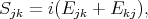 where
where  is the usual canonical basis in
Example 1.1: Consider

A  -invariant Riemannian metric
  in
in  is completely determined by its values in
  , that is, by an inner product
  in
in  invariant under the associated action of
  ([3]). Any inner product in
  , invariant under the associated action of
  has the form
  with
with  definite with respect to the Cartan-Killing form and
  is the Hadamard product or term by term product [3]. The inner product
  admits a natural extension to a bilinear symmetric form on
  We use the same notation
  for this form, as well as for the correspondent complexified form
 -invariance of
  amounts to the Weyl basis being a complex basis of eigenvectors for the action of
  , in other words in
  we have
 | (9) |
with  for
for 
for the real space  the elements of the canonical base
  with
with  , are eigenvectors for the same eigenvalue
  We denote by
  the
the  -invariant metric associated with
  In what follows we will use
  as synonymous of
 -estructures
K. Yano [20] in 1961 introduced  -structure for general manifolds; here we shall be interested in invariant structures. An
  -invariant
  -structure in
  is completely determined by an endomorphism
  , satisfying
  which commutes with the adjoint action of
  We also denote by
  its complexification
  which is diagonalizable with eigenvalues
  , and denote by
  the corresponding eigenspaces. Then we have
  with
with  The
The  -invariance of
  guarantees that
  for all
  with equality when
  is an invariant almost complex structure (see [17]). Thus
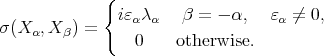
  is determined uniquely by the values
 defined by
  . These values satisfy
  therefore
  is defined by its values in
  In the sequel we allow some abuse of notation and identify the invariant
  -structure
  on
on  with
with  In our invariant context if the
  -structure is an invariant almost complex structure this amounts to
  for all
In what follows we shall simplify notation by suppressing the subscript  in the context of partial flag manifolds.
Denote by  and
and  the complementary projections onto the spaces
  and
and  denoted as
  and
and  , respectively and defined as follow

Since  is an
is an  -structure we have
 | (11) |
where  denote the identity. In other words
  and
and  are complementary projection operators in
Consider an  -estructure
  and
and  ,
,  like below. Then:

 act in
  like an almost complex structure and in
  like the null operator.
 We are interested in studying integrability conditions for  the distributions
  and
and  For this purpose, we need the Nijenhuis tensor which describes the torsion of
  It is given by
![N (X, Y ) = 2([F(X), F (Y )] - F ([F (X), Y ]) - F ([X, F (Y )]) - L([X, Y ]).](/img/revistas/ruma/v47n1/1a10319x.png)
Using Weyl basis properties we get
![1∕2N (X ,X ) = [F (X ),F (X )] - F ([F(X ),X ])+ α β α β α β - F ([X α,F (X β)]) - L([X α,X β] = (- ɛαɛβ + ɛαɛα+ β + ɛβ ɛα+β + ɛ2 )[Xα, Xβ]. α+β](/img/revistas/ruma/v47n1/1a10320x.png)

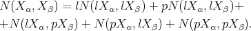
With some simple calculations and using, again, Weyl basis properties we obtain this other identities:
![lN (lX α,lX β) = ɛαɛβɛα+β(ɛα + ɛβ - ɛα+β - ɛαɛ βɛα+β)[Xα, Xβ]; (12) 2 pN (lX α,lX β) = p[F X α,F X β] = ɛαɛβ(ɛα+β - 1)[Xα, Xβ]; (13) N (lX α,lXβ) = F {l(LiepXβF )lX α}; (14) N (pX α,pX β) = lN (pX α,pX β) = (ɛαɛ2 - ɛ2 - ɛ2 + 1)ɛ2 [X α,X β]. (15) β α β α+β](/img/revistas/ruma/v47n1/1a10323x.png)

 Riemannian Connection. Since
  is a naturally reductive homogeneous space its Riemannian connection is given by
![2 ∇X Y = [X, Y ]𝔮Θ + 2U (X, Y),](/img/revistas/ruma/v47n1/1a10327x.png) | (16) |
where  is a symmetric bilinear application
  defined by
![2 ΛΘ(U (X, Y ),Z) = Λ Θ(X, [Y, Z]𝔮Θ) + ΛΘ([Z, X] 𝔮Θ, Y),](/img/revistas/ruma/v47n1/1a10330x.png)
Then the concrete action of the Riemannian connection on the elements of the Weyl basis is given by:
Proposition 6.1. For  let
let  and
and  elements in the Weyl base. Then
 | (17) |
 Kähler form.
 .
.  Derivative in the connection.
![(d∇F )(X ,X ) = ∇ F X - ∇ F X - F [X ,X ] α β (Xλαα-λβ)(βɛα-ɛβ)+Xβλα+β(ɛαα+ɛβ-2ɛαα+β) β = i------------2(λα+β)------------[X α,X β].](/img/revistas/ruma/v47n1/1a10341x.png)
 Lie derivative:
 ![(Lie F )X = F [X ,X ] - [F X ,X ] Xβ α α β α β = i(ɛα+β - ɛβ)[X α,X β].](/img/revistas/ruma/v47n1/1a10343x.png)
7. Graph theoretic description of 
On  invariant
  -structures are in 1:1 correspondence with digraphs
  The correspondence is given by associating with the
  -structure
 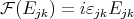 a digraph
  whose vertices are
  and whose arrows are given by the following rules: For


 we may identify an invariant metric
  on
on  with a positive weighting on the edge set
  of the digraph.
 Example 7.1. Again in  let the
  -structure
| |
There exists a complete classification for invariant  -structures on
  (see [5]). Here we present, up to isomorphism, the invariant
  -structures in the case
  this graphs are the most relevant in our present work.
| |
We are now ready to present our characterization of integrability in graph theoretical terms (classical case) or in root terms (general case).
8. Integrability via projections
In this section we will use all the formulas given before to establish integrability conditions for  and for the associated distributions
  and
and  .
.
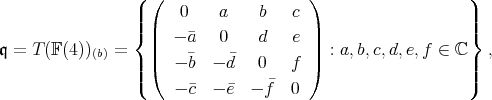
First, we will call the root triple  with
with  whenever
  is called a zero-sum triple. Given an invariant
  -structure
  , each root assumes a sign in
  .
.
Roots triples may then be classified by their sign characteristic, which is a triple 
 where
where  corresponds to the quantity of roots in triple who has
  like its eigenvalue,
  corresponds to the quantity of roots in triple who has
  like its eigenvalue and
  corresponds to the quantity of roots in triple who has
  like its eigenvalue. There are six possible sign characteristics:


By the Frobenious Theorem we know that a distribution is integrable if and only if it is involutive. Thus  is integrable if and only if
 ![l[pX α,pX β] = 0,](/img/revistas/ruma/v47n1/1a10395x.png) that is,
that is,
![l[pX α,pX β] = (ɛ2- 1)(ɛ2 - 1)ɛ2 [X α,X β] = 0. α β α+ β](/img/revistas/ruma/v47n1/1a10396x.png) | (18) |
Theorem 8.1. A necessary and sufficient condition for the distribution  to be integrable is that in
  does not admit triples of type
  In case of
  this condition is equivalent to the associated digraph avoiding the subdigraph (2) in Figure 2.
PROOF. By equation (18)  is not integrable in case where
 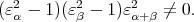 This can only occur when the triple
  is a
is a  -triple. In the classical case, this corresponds the configuration (2) in Figure 2.
Now  is integrable if and only if
 ![p[lX α,lX β] = 0](/img/revistas/ruma/v47n1/1a10407x.png) but
but ![p[lXα, lX β] = (F 2 + 1)[- F 2X α,- F 2Xβ] (19) 2 2 2 = ɛα ɛβ(F + 1)[X α,X β] (20) 2 2 2 = ɛα ɛβ(1 - ɛα+β)[X α,X β]. (21)](/img/revistas/ruma/v47n1/1a10408x.png)
Thus we have the following.
Theorem 8.2. A necessary and sufficient condition for distribution  to be integrable is that in
  does not amit triples of type
  and
and  In case of
  this condition is equivalent to the associated digraph avoiding the subdigraph (3),(4) and (5) in Figure 2.
PROOF. By equation (21)  is not integrable in case
 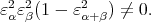 This can only occur when the triple
  is a
is a  -triple or a
  -triple. In the classical case, this corresponds to configurations (3), (4) and (5) in Figure 2.
When  and
and  are integrable, the structure of the submanifolds defined by these distributions and its properties is of interest. We hope to be able to report on this structure in a future communication.
Looking for the integrability of  we need another definition from [7].
Definition 8.3. Assume  integrable and let
  be an arbitrary vector field which is tangent to an integrable manifold of
  It is defined
  Then
Then  is an almost-complex structure on each integral manifold of
 is called partially integrable if both,
  and
and  are integrable.
Theorem 8.4. A necessary and sufficient condition for  be partially integrable is that one of the following equivalent conditions be satisfied:

Using Weyl basis properties the Theorem 8.4 is equivalent to the following.
Theorem 8.5. A necessary and sufficient condition for  to be partially integrable is that in
  does not admit triples of type {0,3,0}, {1,2,0} and
  In the case of
  this condition is equivalent to the associated digraph avoiding the subdigraph (3), (4), (5) and (6) in Figure 2.
PROOF. By Theorem 8.4 is enough to see the conditions  Doing the respective calculations we have
![N (LX α,LX β) = ɛαɛβ(- 1 - ɛβ ɛα+β - ɛαɛα+β + ɛαɛβɛ2α+ β)[X α,X β].](/img/revistas/ruma/v47n1/1a10439x.png)
 is not integrable in case
  this can only occur when the triples are the type in the Theorem. In the classical case this corresponds to configurations (3), (4), (5) and (6) in Figure 2.
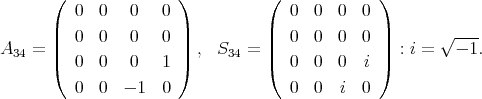
When  and
and  are both integrables, it is possible to choose a local coordinates system such that the operators
  and
and  can be supposed to have the components of the form:
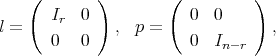
where  is the dimension of the manifold,
  is the rank of
  and
and  means the
  -identity matrix. This coordinate system is called "adapted." Since
  satisfy
  and
and  then in an adapted coordinate system, we can express
  in the following way:
But  means that the components of
  are independent of the coordinates, thus in the next theorem we are interested on this condition in root terms.
Theorem 8.6. Suppose that  and
and  are both integrable and that an adapted coordinate system has been chosen. A necessary and sufficient condition for the local components of
  to be functions independent of the coordinates is that
  in combinatorial terms a necessary and sufficient condition is that in
  does not admit triples of type
  In case of
  this condition is equivalent to the associated digraph avoiding the subdigraphs (4) and (5) in Figure 2.
PROOF. By equation (14) we have the first affirmation and with some calculus we have
![N (lX ,pX ) = ɛ ɛ (1 - ɛ 2)(ɛ ɛ - 1)[X ,X ]. α β α α+β β α α+β α β](/img/revistas/ruma/v47n1/1a10467x.png)
Thus  will be different from zero in case
This can only occur when the triple is  -triple. In the classical case this corresponds to configurations mentioned in the theorem.
When  is an almost complex structure integrability is associated with the existence of canonical coordinate systems, which allows us to consider the manifold as a complex manifold as well is known, integrability is equivalent to
  The following definition in the context of general differential manifolds appears in [7]. Here we present it in the case of flag manifolds.
Definition 8.7. The  -structure
  is called integrable if it satisfies the following three conditions:
 is partially integrable.
 is integrable.
- The components of
 are independent of the coordinates.
With Definition 8.7, we arrive at a general integrability theorem for  -structures.
Theorem 8.8. A necessary and sufficient condition for  to be integrable is that
  Therefore
  is integrable if in
  does not admit triples of type
  and
and  In
In  this condition is equivalent to the associated digraph avoiding the subdigraphs (2), (3), (4), (5) and (6) in figure 2, that is, the associated digraph to
  must be isomorphic to the null digraph or canonical tournament.
PROOF. It is immediate by Definition 8.7 and Theorems 8.1, 8.6 and 8.5. 
Theorem 8.8 is a generalization of the results obtained by Burstall [4] in the case of almost complex structures for classical maximal flag manifolds.
At this point we would like to point out an important connection between integrability and complex structures. It is well known that for a general almost complex structure  on a differential manifold is parallel, namely
  if the manifold with that structure is Kähler. That is, parallelism means that
  is integrable and the manifold is Kähler.
Now a manifold with an  -structure
  will be called Kähler if
Observe that in the case of generalized flag manifolds integrability condition is stronger than Kähler condition, for example, in  the invariant
  -structures to the digraphs (4) and (5) are Kähler but not integrable.
[1] M. Arvanitogeorgos. "An introduction to Lie groups and the geometry of homogeneous spaces". American Mathematical Society Books, Vol. 21 2003. [ Links ]
[2] M. Black. "Harmonic Maps into Homogeneous Spaces". Pitman Research Notes, Math series 255, Longman, Harlow, 1991. [ Links ]
[3] A. Borel, Kählerian coset spaces of semi-simple Lie groups. Proc. Nat. Acad. of Sci. (1954), 40:1147-1151. [ Links ]
[4] F.E. Burstall and S. Salamon. "Tournaments, flags and harmonic maps". Math Ann. 277:249-265, 1987. [ Links ]
[5] N. Cohen, M. Paredes, L. A. B. San Martin, C. J. C. Negreiros, S. Pinzón, f-structures on the classical flag manifold which admit (1,2)-symplectic metrics. Tôhoku Math. J. 57(2) (2005), 262-271. [ Links ]
[6] G. Frobenius, "Uber die Unzerlegbaren diskreten Bewegungsgruppen Sitzungsber". König. Prenss. Acad. Wiss. Berlin 29:654-665, 1911. [ Links ]
[7] S. Ishihara and K. Yano. "On integrability Conditions of a structure  satisfying
  ". Quart. J. Math. Oxford (2), 15:217-222, 1964. [ Links ]
[8] S. Kobayashi and K. Nomizu. Foundations of Differential Geometry, Vol. 1. Interscience Publishers, 1963. [ Links ]
[9] S. Kobayashi and K. Nomizu. Foundations of Differential Geometry, Vol. 2, Interscience Publishers, 1969. [ Links ]
[10] A. Lichnerowicz. "Applications harmoniques et variétés Kähleriennes". Symp. Math. 3 (Bologna), 341-402, 1970. [ Links ]
[11] X. Mo and C.J.C. Negreiros. "Horizontal f-estructures,  -matrices and Equiharmonic moving flags". Relatorio de Pesquisa, Instituto de Matemática, Estatística e Computaçao Científica, Universidade Estadual de Campinas, Brasil, 1999. [ Links ]
[12] Nijenhuis, A. " forming sets of eigenvectors." Indag. Math. 13: 200-212, 1951. [ Links ]
[13] S. Pinzón. Variedades Bandeira, f-Estruturas e Métricas (1,2)-Simpléticas. Ph. D. tesis, Universidade Estadual de Campinas, Brasil, 2003. [ Links ]
[14] J.H. Rawnsley. "f-Structures, f-Twistor Spaces and Harmonic Maps". Lec. Notes in Math., 1164, Springer 1986. [ Links ]
[15] S. Salamon. Harmonic and holomorphic maps. Lec. Notes in Math. 1164, Springer 1986. [ Links ]
[16] L. A. B. San Martin. Algebras de Lie. Campinas, S.P. Editora da Universidade Estadual de Campinas, Brasil, 1999. [ Links ]
[17] L. A. B. San Martin and C. J. C. Negreiros. "Invariant almost Hermitian structures on flag manifolds". Adv. Math. 178 (2003), 277-310. [ Links ]
[18] R.C. de Jesus Silva. Estruturas Quase Hermitianas Invariantes em Espaços Homogêneos de Grupos Semi-simples. Ph. D. tesis, Universidade Estadual de Campinas, Brasil, 2003.. [ Links ]
[19] J. A. Wolf and A. Gray. "Homogeneous spaces defined by Lie group automorphisms, II". J. Diff. Geom. 2:115-159, 1968. [ Links ]
[20] K. Yano. "On a structure defined by a tensor field of type (1,1) satisfying  ". Tensor 14:99-109, 1963. [ Links ]
Sofía Pinzón
Escuela de Matemáticas,
Universidad Industrial de Santander,
A.A. 678, Bucaramanga, Colombia.
Recibido: 30 de septiembre de 2005
Aceptado: 18 de septiembre de 2006

