A short survey on biharmonic maps between Riemannian manifolds

S. Montaldo and C. Oniciuc

2000 Mathematics Subject Classification. 58E20.

Key words and phrases. Harmonic and biharmonic maps.

The first author was supported by Regione Autonoma Sardegna (Italy). The second author was supported by a CNR-NATO (Italy) fellowship, and by the Grant At, 73/2005, CNCSIS (Romania)

1. Introduction

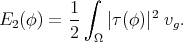
Let be the space of smooth maps between two Riemannian manifolds. A map 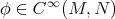is called harmonic if it is a critical point of the energy functional

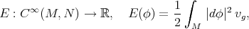
and is characterized by the vanishing of the first tension field 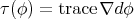. In the same vein, if we denote by the space of Riemannian immersions in , then a Riemannian immersion is called minimal if it is a critical point of the volume functional

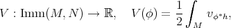
and the corresponding Euler-Lagrange equation is , where is the mean curvature vector field.

If is a Riemannian immersion, then it is a critical point of the bienergy in if and only if it is a minimal immersion [26]. Thus, in order to study minimal immersions one can look at harmonic Riemannian immersions.

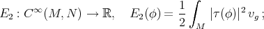
A natural generalization of harmonic maps and minimal immersions can be given by considering the functionals obtained integrating the square of the norm of the tension field or of the mean curvature vector field, respectively. More precisely:

• biharmonic maps are the critical points of the bienergy functional

  

• Willmore immersions are the critical points of the Willmore functional

  

  where is the sectional curvature of restricted to the image of .

While the above variational problems are natural generalizations of harmonic maps and minimal immersions, biharmonic Riemannian immersions do not recover Willmore immersions, even when the ambient space is . Therefore, the two generalizations give rise to different variational problems.

In a different setting, in [19], B.Y. Chen defined biharmonic submanifolds of the Euclidean space as those with harmonic mean curvature vector field, that is , where is the rough Laplacian. If we apply the definition of biharmonic maps to Riemannian immersions into the Euclidean space we recover Chen's notion of biharmonic submanifolds. Thus biharmonic Riemannian immersions can also be thought as a generalization of Chen's biharmonic submanifolds.

In the last decade there has been a growing interest in the theory of biharmonic maps which can be divided in two main research directions. On the one side, the differential geometric aspect has driven attention to the construction of examples and classification results; this is the face of biharmonic maps we shall try to report. The other side is the analytic aspect from the point of view of PDE: biharmonic maps are solutions of a fourth order strongly elliptic semilinear PDE. We shall not report on this aspect and we refer the reader to [18, 35, 36, 55, 56, 57] and the references therein.

The differential geometric aspect of biharmonic submanifolds was also studied in the semi-Riemannian case. We shall not discuss this case, although it is very rich in examples, and we refer the reader to [20] and the references therein.

We mention some other reasons that should encourage the study of biharmonic maps.

• The theory of biharmonic functions is an old and rich subject: they have been studied since 1862 by Maxwell and Airy to describe a mathematical model of elasticity; the theory of polyharmonic functions was later on developed, for example, by E. Almansi, T. Levi-Civita and M. Nicolescu. Recently, biharmonic functions on Riemannian manifolds were studied by R. Caddeo and L. Vanhecke [10, 17], L. Sario et al. [52], and others.
• The identity map of a Riemannian manifold is trivially a harmonic map, but in most cases is not stable (local minimum), for example consider . In contrast, the identity map, as a biharmonic map, is always stable, in fact an absolute minimum of the energy.
• Harmonic maps do not always exists, for instance, J. Eells and J.C. Wood showed in [27] that there exists no harmonic map from to (whatever the metrics chosen) in the homotopy class of Brower degree . We expect biharmonic maps to succeed where harmonic maps have failed.

In this short survey we try to report on the theory of biharmonic maps between Riemannian manifolds, conscious that we might have not included all known results in the literature.

Table of Contents

2. The biharmonic equation
3. Non-existence results
    3.1. Riemannian immersions
    3.2. Submanifolds of
    3.3. Riemannian submersions
4. Biharmonic Riemannian immersions
    4.1. Biharmonic curves on surfaces
    4.2. Biharmonic curves of the Heisenberg group
    4.3. The biharmonic submanifolds of
    4.4. Biharmonic submanifolds of
    4.5. Biharmonic submanifolds in Sasakian space forms
5. Biharmonic Riemannian submersions
6. Biharmonic maps between Euclidean spaces
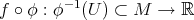
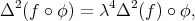
7. Biharmonic maps and conformal changes
    7.1. Conformal change on the domain
    7.2. Conformal change on the codomain
8. Biharmonic morphisms
9. The second variation of biharmonic maps

Acknowledgements. The first author wishes to thank the organizers of the "II Workshop in Differential Geometry - Córdoba - June 2005" for their exquisite hospitality and the opportunity of presenting a lecture. The second author wishes to thank Renzo Caddeo and the Dipartimento di Matematica e Informatica, Università di Cagliari, for hospitality during the preparation of this paper.

2. The biharmonic equation

Let be a smooth map, then, for a compact subset , the energy of is defined by

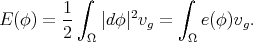
Critical points of the energy, for any compact subset , are called harmonic maps and the corresponding Euler-Lagrange equation is

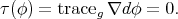
The equation is called the harmonic equation and, in local coordinates on and on , takes the familiar form

where are the Christoffel symbols of and 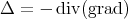is the Beltrami-Laplace operator on .

A smooth map is biharmonic if it is a critical point, for any compact subset , of the bienergy functional

We will now derive the biharmonic equation, that is the Euler-Lagrange equation associated to the bienergy. For simplicity of exposition we will perform the calculation for smooth maps 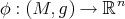, defined by , with compact. In this case we have

(2.1)

To compute the corresponding Euler-Lagrange equation, let be a one-parameter smooth variation of in the direction of a vector field on and denote with the operator . We have

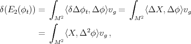
where in the last equality we have used that is self-adjoint. Since 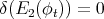, for any vector field , we conclude that is biharmonic if and only if

Moreover, if is a Riemannian immersion, then, using Beltrami equation , we have that is biharmonic if and only if

Therefore, as mentioned in the introduction, we recover Chen's definition of biharmonic submanifolds in .

For a smooth map the Euler-Lagrange equation associated to the bienergy becomes more complicated and, as one would expect, it involves the curvature of the codomain. More precisely, a smooth map is biharmonic if it satisfies the following biharmonic equation

where 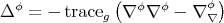is the rough Laplacian on sections of and is the curvature operator on .

From the expression of the bitension field it is clear that a harmonic map () is automatically a biharmonic map, in fact a minimum of the bienergy.

We call a non-harmonic biharmonic map a proper biharmonic map.

3. Non-existence results

As we have just seen, a harmonic map is biharmonic, so a basic question in the theory is to understand under what conditions the converse is true. A first general answer to this problem, proved by G.Y. Jiang, is

Theorem 3.1 ([33, 34]). Let be a smooth map. If is compact, orientable and , then is biharmonic if and only if it is harmonic.

Jiang's theorem is a direct application of the Weitzenböck formula. In fact, if is biharmonic, the Weitzenböck formula and give

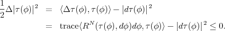
Then, since is compact, by the maximal principle, we find that . Now using the identity

we deduce that and, after integration, we conclude.

3.1. Riemannian immersions. If is not compact, then the above argument can be used with the extra assumption that is a Riemannian immersion and that the norm of is constant, as was shown by C. Oniciuc in

Theorem 3.2 ([44]). Let be a Riemannian immersion. If is constant and , then is biharmonic if and only if it is minimal.

The curvature condition in Theorems 3.1 and 3.2 can be weakened in the case of codimension one, that is . We have

Theorem 3.3 ([44]). Let be a Riemannian immersion with and .

• If is compact and orientable, then is biharmonic if and only if it is minimal.
• If is constant, then is biharmonic if and only if it is minimal.

3.2. Submanifolds of . Let be a manifold with constant sectional curvature , a submanifold of and denote by the canonical inclusion. In this case the tension and bitension fields assume the following form

If , there are strong restrictions on the existence of proper biharmonic submanifolds in . If is compact, then there exists no proper biharmonic Riemannian immersion from into . In fact, from Theorem 3.1, should be minimal. If is not compact and is a proper biharmonic map then, from Theorem 3.2, cannot be constant.

If , as we shall see in Sections 4.3 and 4.4, we do have examples of compact proper biharmonic submanifolds.

The main tool in the study of biharmonic submanifolds of is the decomposition of the bitension field in its tangential and normal components. Then, asking that both components are identically zero, we conclude that the canonical inclusion is biharmonic if and only if

(3.1)

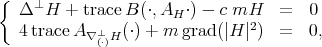
where is the second fundamental form of in , the shape operator, the normal connection and the Laplacian in the normal bundle of .

Equation (3.1) was used by B.Y. Chen, for , and by R. Caddeo, S. Montaldo and C. Oniciuc, for , to prove that in the case of biharmonic surfaces in , the mean curvature must be constant, thus

Theorem 3.4 ([19, 21, 12]). Let be a surface of . Then is biharmonic if and only if it is minimal.

For higher dimensional cases it is not known whether there exist proper biharmonic submanifolds of , although, for , partial results have been obtained. For instance:

• Every biharmonic curve of is an open part of a straight line [24].
• Every biharmonic submanifold of finite type in is minimal [24].
• There exists no proper biharmonic hypersurface of with at most two principal curvatures [24].
• Let be a pseudo-umbilical submanifold of . If , then is biharmonic if and only if minimal [24].
• Let be a hypersurface of . Then is biharmonic if and only if minimal [30].
• Any submanifold of cannot be biharmonic in [19].
• Let be a pseudo-umbilical submanifold of . If , then is biharmonic if and only if minimal [12].

All these results suggested the following

Generalized Chen's Conjecture: Biharmonic submanifolds of a manifold with are minimal.

3.3. Riemannian submersions. Let be a Riemannian submersion with basic tension field. Then the bitension field, computed in [44], is

(3.2)

Using this formula we find some non-existence results which are, in some sense, dual to those for Riemannian immersions. They can be stated as follows:

Proposition 3.5 ([44]). A biharmonic Riemannian submersion with basic tension field is harmonic in the following cases:

• if is compact, orientable and ;
• if and is constant;
• if is compact and .

4. Biharmonic Riemannian immersions

In this section we report on the known examples of proper biharmonic Riemannian immersions. Of course, the first and easiest examples can be found looking at differentiable curves in a Riemannian manifold. This is the first class we shall describe.

Let be a curve parametrized by arc length from an open interval to a Riemannian manifold. In this case the tension field becomes , and the biharmonic equation reduces to

(4.1)

To describe geometrically Equation (4.1) let us recall the definition of the Frenet frame.

Definition 4.1 (See, for example, [37]). The Frenet frame associated to a curve , parametrized by arc length, is the orthonormalisation of the -uple 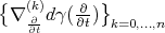, described by:

where the functions are called the curvatures of and is the connection on the pull-back bundle . Note that is the unit tangent vector field along the curve.

We point out that when the dimension of is , the first curvature is replaced by the signed curvature.

Using the Frenet frame, we get that a curve is proper () biharmonic if and only if

(4.2)

4.1. Biharmonic curves on surfaces. Let be an oriented surface and let be a differentiable curve parametrized by arc length. Then Equation (4.2) reduces to

where is the curvature (with sign) of and is the Gauss curvature of the surface.

As an immediate consequence we have:

Proposition 4.2 ([14]). Let be a proper biharmonic curve on an oriented surface . Then, along , the Gauss curvature must be constant, positive and equal to the square of the geodesic curvature of . Therefore, if has non-positive Gauss curvature, any biharmonic curve is a geodesic of .

Proposition 4.2 gives a positive answer to the generalized Chen's conjecture.

Now, let be a curve in the -plane and consider the surface of revolution, obtained by rotating this curve about the -axis, with the standard parametrization

where is the rotation angle. Assuming that is parametrized by arc length, we have

Proposition 4.3 ([14]). A parallel is biharmonic if and only if satisfies the equation

Example 4.4 (Torus). On a torus of revolution with its standard parametrization

the biharmonic parallels are

Example 4.5 (Sphere). There is a geometric way to understand the behaviour of biharmonic curves on a sphere. In fact, the torsion and curvature (without sign) of , seen in the ambient space , satisfy 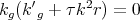. From this we see that is a proper biharmonic curve if and only if and , i.e. is the circle of radius .

For more examples see [14, 15].

4.2. Biharmonic curves of the Heisenberg group . The Heisenberg group can be seen as the Euclidean space endowed with the multiplication

and with the left-invariant Riemannian metric given by

(4.3)

Let be a differentiable curve parametrized by arc length. Then, from (4.2), is a proper biharmonic curve if and only if

(4.4)

where , , and . Here is the left-invariant orthonormal basis with respect to the metric (4.3).

By analogy with curves in , we use the name helix for a curve in a Riemannian manifold having both geodesic curvature and geodesic torsion constant.

Using System (4.4), in [16], R. Caddeo, C. Oniciuc and P. Piu showed that a proper biharmonic curve in is a helix and gave their explicit parametrizations, as shown in the following

Theorem 4.6 ([16]). The parametric equations of all proper biharmonic curves of are

(4.5)

where , and .

Geometrically, proper biharmonic curves in can be obtained as the intersection of a minimal helicoid with a round cylinder. Moreover, they are geodesic of this round cylinder.

The above method can be extended to study biharmonic curves in Cartan-Vranceanu three-manifolds (), where if , if , and the Riemannian metric is defined by

(4.6)

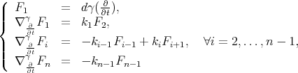
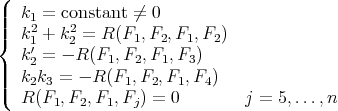
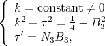
This two-parameter family of metrics reduces to the Heisenberg metric for and . The system for proper biharmonic curves corresponding to the metric can be obtained by using the same techniques, and turns out to be

(4.7)

System 4.7 also implies that the proper biharmonic curves of are helices [13]. The explicit parametrization of proper biharmonic curves of was given in [23], for , and in [13] in general.

We point out that biharmonic curves were studied in other spaces which are generalizations of the above cases. For example:

• In [28], D. Fetcu studied biharmonic curves in the dimensional Heisenberg group and obtained two families of proper biharmonic curves.
• A. Balmuş studied, in [6], the biharmonic curves on Berger spheres , obtaining their explicit parametric equations.

4.3. The biharmonic submanifolds of . In [11] the authors give a complete classification of the proper biharmonic submanifolds of .

Using System(4.2) it was first proved that the proper biharmonic curves are the helices with . If we look at as a curve in , the biharmonic condition can be expressed as

(4.8)

Now, by integration of (4.8), we obtain

Theorem 4.7 ([11],[8]). Let be a curve parametrized by arc length. Then it is proper biharmonic if and only if it is either the circle of radius , or a geodesic of the Clifford torus 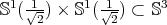with slope different from .

As to proper biharmonic surfaces of the three-dimensional sphere, one can first prove that Equation (3.1) implies the following

Theorem 4.8 ([11]). Let be a surface of . Then it is proper biharmonic if and only if is constant and .

The classification of constant mean curvature surfaces in with is known, in fact we have

Theorem 4.9 ([11],[31]). Let be a surface of with constant mean curvature and .

• If is not compact, then locally it is a piece of either a hypersphere or a torus .
• If is compact and orientable, then it is either or .

Now, since the Clifford torus is minimal in , we can state:

Theorem 4.10 ([11]). Let be a proper biharmonic surface of .

• If is not compact, then it is locally a piece of .
• If is compact and orientable, then it is .

4.4. Biharmonic submanifolds of . We start describing some basic examples of proper biharmonic submanifolds of .

Let , , . Up to a homothetic transformation, is the canonical inclusion of the hypersphere in . A simple calculation shows that . Derivating with respect to we find that if and only if .

This simple argument shows that is a good candidate for proper biharmonic submanifold of if . It is not difficult to show that, indeed, the bitension field of is zero, proving that it is the only proper biharmonic hypersphere of .

To explain the next example we first note that, from (3.1), we have

Proposition 4.11. Let be a non-minimal hypersurface of with parallel mean curvature, i.e. the norm of is constant. Then is a proper biharmonic submanifold if and only if .

Let be two positive integers such that , and let be two positive real numbers such that . Then the generalized Clifford torus is a hypersurface of . A simple calculation shows that

We thus have

Example 4.12 ([33, 34]).

1. If , then is a proper biharmonic submanifold of if and only if .
2. If , then the following statements are equivalent:
   • is a biharmonic submanifold of
   • is a minimal submanifold of
   • .

The submanifolds and the generalized Clifford torus are the only known examples of proper biharmonic hypersurfaces of . As we have seen in Theorem 4.10, for , the hypersphere is the only one.

Open problem: classify all proper biharmonic hypersurfaces of .

The situation seems much richer if the codimension is greater than one. We shall present a construction of proper biharmonic submanifolds in . Let be a submanifold of . Then can be seen as a submanifold of and we have

Theorem 4.13 ([12],[42]). Assume that is a submanifold of . Then is a proper biharmonic submanifold of if and only if it is minimal in .

Theorem 4.13 is a useful tool to construct examples of proper biharmonic submanifolds. For instance, using a well known result of H.B. Lawson [38], we have

Theorem 4.14 ([12]). There exist closed orientable embedded proper biharmonic surfaces of arbitrary genus in .

This shows the existence of an abundance of proper biharmonic surfaces in , in contrast with the case of .

The biharmonic submanifolds that we have produced so far are all pseudo-umbilical, i.e. . We now want to give examples of biharmonic submanifolds of that are not of this type.

With this aim, let , be two positive integers such that , and let , be two positive real numbers such that . Let be a minimal submanifold of , of dimension , with , and let be a minimal submanifold of , of dimension , with . We have:

Theorem 4.15 ([12]). The manifold is a proper biharmonic submanifold of if and only if and .

If is a submanifold of with , then it is possible to give a partial classification. In fact we have

Theorem 4.16 ([48]). Let be a submanifold of such that is constant.

• If , then is never biharmonic.
• If , then is biharmonic if and only if it is pseudo-umbilical and , i.e. is a minimal submanifold of .

As an immediate consequence we have

Corollary 4.17 ([48]). If is a compact orientable hypersurface of with , then is proper biharmonic if and only if .

Another partial classification for compact hypersurfaces in was given in [22], in terms of the length of the second fundamental form and of the sign of the sectional curvature.

We end this section presenting two classes of proper biharmonic curves of

Proposition 4.18 ([12]).

1. The circles where , , are constant orthogonal vectors of with , are proper biharmonic curves of .
2. The curves where , , , are constant orthogonal vectors of with , and , , are proper biharmonic of .

4.5. Biharmonic submanifolds in Sasakian space forms. A "generalization" of Riemannian manifolds with constant sectional curvature is that of Sasakian space forms. First, recall that is a contact Riemannian manifold if: is a -dimensional manifold; is an one-form satisfying ; is the vector field defined by and ; is an endomorphism field; is a Riemannian metric on such that, ,

• 
• 
• .

A contact Riemannian manifold is a Sasaki manifold if

If the sectional curvature is constant on all -invariant tangent -planes of , then is called of constant holomorphic sectional curvature. Moreover, if a Sasaki manifold is connected, complete and of constant holomorphic sectional curvature, then it is called a Sasakian space form. We have the following classification.

Theorem 4.19 ([9]). A simply connected three-dimensional Sasakian space form is isomorphic to one of the following:

• the special unitary group
• the Heisenberg group
• the universal covering group of .

In particular, a simply connected three-dimensional Sasakian space form of constant holomorphic sectional curvature is isometric to .

In [32], J. Inoguchi classified proper biharmonic Legendre curves and Hopf cylinders in three-dimensional Sasakian space forms. To state Inoguchi results we recall that:

• a curve parametrized by arc length is Legendre if ;
• a Hopf cylinder is , where is the projection of onto the orbit space determined by the action of the one-parameter group of isometries generated by , when the action is simply transitive.

Theorem 4.20 ([32]). Let be a Sasakian space form of constant holomorphic sectional curvature and a biharmonic Legendre curve parametrized by arclength.

• If , then is a Legendre geodesic.
• If , then is a Legendre geodesic or a Legendre helix of curvature .

Theorem 4.21 ([32]). Let be a biharmonic Hopf cylinder in a Sasakian space form.

• If , then is a geodesic.
• If , then is a geodesic or a Riemannian circle of curvature .

In particular, there exist proper biharmonic Hopf cylinders in Sasakian space forms of holomorphic sectional curvature greater than .

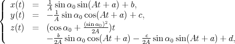
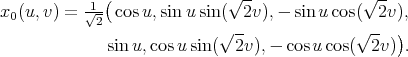
T. Sasahara classified, in [53], proper biharmonic Legendre surfaces in Sasakian space forms and, in the case when the ambient space is the unit -dimensional sphere , he obtained their explicit representations.

Theorem 4.22 ([53]). Let be a proper biharmonic Legendre immersion. Then the position vector field of in is given by:

Other results on biharmonic Legendre curves and biharmonic anti-invariant surfaces in Sasakian space forms and -manifolds were obtained in [1, 2].

5. Biharmonic Riemannian submersions

In this section we discuss some examples of proper biharmonic Riemannian submersions. From the expression of the bitension field (3.2) we have immediately the following

Theorem 5.1 ([44]). Let be a Riemannian submersion with basic, non-zero, tension field. Then is proper biharmonic if:

• ;
• is a unit Killing vector field on .

Theorem 5.1 was used in [44] to construct examples of proper biharmonic Riemannian submersions. These examples are projections from the tangent bundle of a Riemannian manifold endowed with a "Sasaki type" metric. Indeed, let be an -dimensional Riemannian manifold and let be its tangent bundle. We denote by the vertical distribution on defined by , . We consider a nonlinear connection on defined by the distribution on , complementary to , i.e. , . For any induced local chart on we have a local adapted frame in defined by the local vector fields

where the local functions are the connection coefficients of the nonlinear connection defined by . If we endow with the Riemannian metric defined by

then the canonical projection is a Riemannian submersion. (For more details on the metrics on the tangent bundle see, for example, [49].) The biharmonicity of the map depends on the choice of the connection coefficients . For suitable choices we have:

Proposition 5.2 ([44]).

• Let be an unit Killing vector field and let be a projective change of the Levi-Civita connection on . Then is a proper biharmonic map.
• Let , be an affine function and let , be a conformal change of the connection . Then is a proper biharmonic map.

Another important class of biharmonic Riemannian submersions was described in [7] and it is descried as follows. Let and be Riemannian manifolds and denote by their warped product with respect to a positive function on , then the projection is a Riemannian submersion with . When is affine, is Killing of constant norm, hence is biharmonic.

6. Biharmonic maps between Euclidean spaces

Let , be a smooth map. Then, the bitension field assumes the simple expression . Thus, a map is biharmonic if and only if its component functions are biharmonic.

If we want proper solutions defined everywhere, then we can take polynomial solutions of degree three. If we look for maps which are not defined everywhere, then there are interesting classes of examples. One of these can be described as follows.

A smooth map is axially symmetric if there exist a map and a function such that, for ,

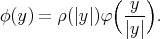
Assume that the map is not constant. An axially symmetric map is harmonic if and only if is an eigenmap of eigenvalue (see [25] for the definition of eigenmaps) and

(6.1)

where and with .

The biharmonicity of axially symmetric maps was discussed in [7], where the authors give the following classification.

Theorem 6.1 ([7]). Let be an axially symmetric map and assume that is an eigenmap of eigenvalue .

1. If , then
   • for , can not be biharmonic.
   • for , is proper biharmonic if and only if is an eigenmap of homogeneous degree .
   • for , is proper biharmonic if and only if is an eigenmap of homogeneous degree .
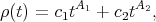
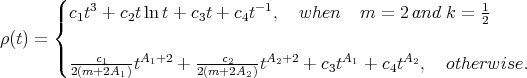
2. If , then is proper biharmonic if and only if

   (6.2)

   where and arbitrary such that takes values in .

Example 6.2. An important class of axially symmetric diffeomorphisms of is given by

which, for , provides the well known Kelvin transformation. For these maps, and is the identity map. An easy computation shows that is harmonic if and only if .

Using (6.2) it follows that is proper biharmonic if and only if . For this result was first obtained in [3].

We also note that the proper biharmonic map , , is harmonic with respect to the conformal metric on the domain given by . This property is similar to that of the Kelvin transformation proved by B. Fuglede in [29].

7. Biharmonic maps and conformal changes

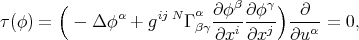
7.1. Conformal change on the domain. Let be a harmonic map. Consider a conformal change of the domain metric, i.e. for some smooth function .

If , from the conformal invariance of the energy, the map remains harmonic. If , then does not remain, necessarily, harmonic. Therefore, it is reasonable to seek under what conditions on the function the map is biharmonic.

This problem was attacked in [3], where P. Baird and D. Kamissoko first proved the following general result.

Proposition 7.1 ([3]). Let , be a harmonic map. Let be a metric conformally equivalent to . Then is biharmonic if and only if

If is the identity map , we call a conformally equivalent metric , for which becomes biharmonic, a biharmonic metric with respect to .

Applying the maximum principle we have

Theorem 7.2 ([3]). Let , , be a compact manifold of negative Ricci curvature. Then there is no biharmonic metric conformally related to other than a constant multiple of .

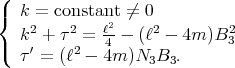
There is a surprising connection between biharmonic metrics and isoparametric functions. We recall that a smooth function is called isoparametric if, for each where , there are real functions and such that

on some neighbourhood of . The above mentioned link is provided by the following

Theorem 7.3 ([3]). Let , , be an Einstein manifold. Let be a biharmonic metric conformally equivalent to . Then the function is isoparametric.

Conversely, let be an isoparametric function, then away from critical points of , there is a reparametrization such that is a biharmonic metric.

7.2. Conformal change on the codomain. Let be a harmonic map. Consider the "dual problem", i.e. a conformal change of the codomain metric. In this case the analogous of Proposition 7.1 is more complicated and we shall review only on some special situations.

If is the identity map, then it is proved, in [5], that is biharmonic if and only if

This equation was used in [5] to prove similar results to Theorem 7.3, for the conformal change of the metric on the codomain.

In a similar setting, in [46, 47], C. Oniciuc constructed new examples of biharmonic maps deforming the metric on a sphere. More precisely, let be the -dimensional sphere endowed with the conformal modified metric , where is the canonical metric on and . Let be the equatorial sphere of . Then the inclusion is a proper biharmonic map.

This result was generalized in

Theorem 7.4 ([46, 47]). Let be a minimal submanifold of . Then is a proper biharmonic submanifold of .

Observe that even a geodesic will not remain harmonic after a conformal change of the metric on , unless the conformal factor is constant. As to biharmonicity of we have the following.

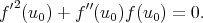
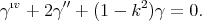
Theorem 7.5 ([39]). Let be a Riemannian manifold. Fix a point and let be a non-constant function, depending only on the geodesic distance from , which is a solution of the following ODE:

Then any geodesic such that becomes a proper biharmonic curve .

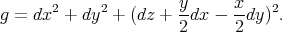
For example, take and , where is the distance from the origin. Then any straight line on the flat turns to a biharmonic curve on , which is the metric, in local isothermal coordinates, of the Enneper minimal surface.

8. Biharmonic morphisms

In analogy with the case of harmonic morphisms (see [4]) the definition of biharmonic morphisms can be formulated as follows.

Definition 8.1. A map is a biharmonic morphism if for any biharmonic function , its pull-back by , , is a biharmonic function.

In [40] E. Loubeau and Y.-L. Ou gave the characterization of the biharmonic morphisms showing that a map is a biharmonic morphism if and only if it is a horizontally weakly conformal biharmonic map and its dilation satisfies a certain technical condition.

A more direct characterization is

Theorem 8.2 ([50, 40]). A map is a biharmonic morphism if and only if there exists a function such that

for all functions .

If is compact, the notion of biharmonic morphisms becomes trivial, in fact we have

Theorem 8.3 ([40]). Let be a non-constant map. If is compact, then is a biharmonic morphism if and only if it is a harmonic morphism of constant dilation, hence a homothetic submersion with minimal fibers.

In [51], Y.-L. Ou, using the theory of -harmonic morphisms, proved the following properties.

Theorem 8.4 ([51]). The radial projection 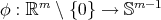, , is a biharmonic morphism if and only if .

Theorem 8.5 ([51]). The projection 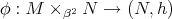, , of a warped product onto its second factor is a biharmonic morphism if and only if is a harmonic function on .

In the case of polynomial biharmonic morphisms between Euclidean spaces there is a full classification.

Theorem 8.6 ([51]). Let be a polynomial biharmonic morphism, i.e. a biharmonic morphism whose component functions are polynomials, with . Then is an orthogonal projection followed by a homothety.

9. The second variation of biharmonic maps

The second variation formula for the bienergy functional was obtained, in a general setting, by G.Y. Jiang in [34]. For biharmonic maps in Euclidean spheres, the second variation formula takes a simpler expression.

Theorem 9.1 ([45]). Let be a biharmonic map. Then the Hessian of the bienergy at is given by

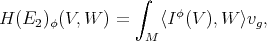
where

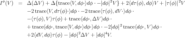
Although the expression of the operator is rather complicated, in some particular cases it becomes easy to study.

In the instance when is the identity map of , has the expression

and we can immediately deduce

Theorem 9.2 ([45]). The identity map is biharmonic stable and

1. if , then ;
2. if , then .

A large class of biharmonic maps for which it is possible to study the Hessian is obtained using the following generalization of Theorem 4.13.

Theorem 9.3 ([42]). Let be an orientable compact manifold and the canonical inclusion. If is a non-constant map, then is proper biharmonic if and only if is harmonic and is constant.

Remark 9.4. All the biharmonic maps constructed using Theorem 9.3 are unstable. To see this, let , , , the map defined in Section 4.4. Then

Thus the problem is to describe qualitatively their index and nullity.

Theorem 9.5 ([41]). Let be a minimal immersion. The nullity of the biharmonic map is bounded from below by the dimension of .

When is the identity map of we have

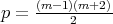
Theorem 9.6 ([41],[8]). The biharmonic index of the canonical inclusion is exactly , and its nullity is .

Proposition 9.7 ([43]). Let be a minimal immersion, . Then

1. if either , or and ;
2. if and .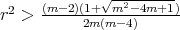

When is the minimal generalized Veronese map we get

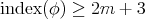
Corollary 9.8 ([41]). The biharmonic map derived from the generalized Veronese map 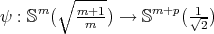, , has index at least , when , and at least , when .

In Theorem 9.6 and Proposition 9.7 the map was a minimal immersion. We shall consider now the case of harmonic Riemannian submersions, and choose for the Hopf map.

Theorem 9.9 ([42]). The index of the biharmonic map is at least , while its nullity is bounded from below by .

We note that, for the above results, the authors described explicitly the spaces where is negative definite or vanishes.

For the case of surfaces in Sasakian space forms, T. Sasahara, considering a variational vector field parallel to , gave a sufficient condition for proper biharmonic Legendre submanifolds into an arbitrary Sasakian space form to be unstable. This condition is expressed in terms of the mean curvature vector field and of the second fundamental form of the submanifold. In particular

Theorem 9.10 ([54]). The biharmonic Legendre curves and surfaces in Sasakian space forms are unstable.

References

[1]    K. Arslan, R. Ezentas, C. Murathan, T. Sasahara. Biharmonic anti-invariant submanifolds in Sasakian space forms. Beitrage Algebra Geom., to appear.        [ Links ]

[2]    K. Arslan, R. Ezentas, C. Murathan, T. Sasahara. Biharmonic submanifolds in 3-dimensional -manifolds. Internat. J. Math. Math. Sci., 22 (2005), 3575-3586.        [ Links ]

[3]    P. Baird, D. Kamissoko. On constructing biharmonic maps and metrics. Ann. Global Anal. Geom. 23 (2003), 65-75.        [ Links ]

[4]    P. Baird, J.C. Wood. Harmonic Morphisms between Riemannian Manifolds. Oxford Science Publications, 2003.        [ Links ]

[5]    A. Balmuş. Biharmonic properties and conformal changes. An. Stiint. Univ. Al.I. Cuza Iasi Mat. (N.S.) 50 (2004), 361-372.        [ Links ]

[6]    A. Balmuş. On the biharmonic curves of the Euclidian and Berger 3-dimensional spheres. Sci. Ann. Univ. Agric. Sci. Vet. Med. 47 (2004), 87-96.        [ Links ]

[7]    A. Balmuş, S. Montaldo, C. Oniciuc. Biharmonic maps between warped product manifolds, J. Geom. Phys. 57 (2007), 449-466.        [ Links ]

[8]    A. Balmuş, C. Oniciuc. Some remarks on the biharmonic submanifolds of and their stability. An. Stiint. Univ. Al.I. Cuza Iasi, Mat. (N.S), 51 (2005), 171-190.        [ Links ]

[9]    J. Berndt, F. Tricerri, L. Vanhecke. Generalized Heisenberg groups and Damek-Ricci harmonic spaces. Lecture Notes in Mathematics, 1598. Springer-Verlag, Berlin, 1995.        [ Links ]

[10]    R. Caddeo. Riemannian manifolds on which the distance function is biharmonic. Rend. Sem. Mat. Univ. Politec. Torino, 40 (1982), 93-101.        [ Links ]

[11]    R. Caddeo, S. Montaldo, C. Oniciuc. Biharmonic submanifolds of . Int. J. Math., 12 (2001), 867-876.        [ Links ]

[12]    R. Caddeo, S. Montaldo, C. Oniciuc. Biharmonic submanifolds in spheres. Israel J. Math., 130 (2002), 109-123.        [ Links ]

[13]    R. Caddeo, S. Montaldo, C. Oniciuc, P. Piu. The classification of biharmonic curves of Cartan-Vranceanu -dimensional spaces. Modern trends in geometry and topology, Cluj Univ. Press, Cluj-Napoca (2006), 121-131.        [ Links ]

[14]    R. Caddeo, S. Montaldo, P. Piu. Biharmonic curves on a surface. Rend. Mat. Appl., 21 (2001), 143-157.        [ Links ]

[15]    R. Caddeo, S. Montaldo, P. Piu. On Biharmonic Maps. Contemporary Mathematics, 288 (2001), 286-290.        [ Links ]

[16]    R. Caddeo, C. Oniciuc, P. Piu. Explicit formulas for non-geodesic biharmonic curves of the Heisenberg group. Rend. Sem. Mat. Univ. Politec. Torino, 62 (2004), 265-278.        [ Links ]

[17]    R. Caddeo, L. Vanhecke. Does " on a Riemannian manifold" imply flatness? Period. Math. Hungar., 17 (1986), 109-117.        [ Links ]

[18]    S.-Y. A. Chang, L. Wang, P.C. Yang. A regularity theory of biharmonic maps. Comm. Pure Appl. Math., 52 (1999), 1113-1137.        [ Links ]

[19]    B.-Y. Chen. Some open problems and conjectures on submanifolds of finite type. Soochow J. Math., 17 (1991), 169-188.        [ Links ]

[20]    B.-Y. Chen. A report on submanifolds of finite type. Soochow J. Math., 22 (1996), 117-337.        [ Links ]

[21]    B.-Y. Chen, S. Ishikawa. Biharmonic pseudo-Riemannian submanifolds in pseudo-Euclidean spaces. Kyushu J. Math., 52 (1998), 167-185.        [ Links ]

[22]    J.H. Chen. Compact 2-harmonic hypersurfaces in . Acta Math. Sinica, 36 (1993), 341-347.        [ Links ]

[23]    J.T. Cho, J. Inoguchi, J.-E. Lee. Biharmonic curves in 3-dimensional Saskian space forms. Ann. Mat. Pura Appl., to appear.        [ Links ]

[24]    I. Dimitric. Submanifolds of with harmonic mean curvature vector. Bull. Inst. Math. Acad. Sinica, 20 (1992), 53-65.        [ Links ]

[25]    J. Eells, A. Ratto. Harmonic Maps and Minimal Immersions with Symmetries. Princeton University Press, 1993.        [ Links ]

[26]    J. Eells, J.H. Sampson. Harmonic mappings of Riemannian manifolds. Amer. J. Math., 86 (1964), 109-160.        [ Links ]

[27]    J. Eells, J.C. Wood. Restrictions on harmonic maps of surfaces. Topology, 15 (1976), 263-266.        [ Links ]

[28]    D. Fetcu. Biharmonic curves in the generalized Heisenberg group. Beiträge Algebra Geom., 46 (2005), 513-521.        [ Links ]

[29]    B. Fuglede. Harmonic morphisms between Riemannian manifolds. Ann. Inst. Fourier (Grenoble) 28 (1978), 107-144.        [ Links ]

[30]    T. Hasanis, T. Vlachos. Hypersurfaces in with harmonic mean curvature vector field. Math. Nachr., 172 (1995), 145-169.        [ Links ]

[31]    Z.H. Hou. Hypersurfaces in a sphere with constant mean curvature. Proc. Amer. Math. Soc. 125 (1997), 1193-1196.        [ Links ]

[32]    J. Inoguchi. Submanifolds with harmonic mean curvature in contact 3-manifolds. Colloq. Math., 100 (2004), 163-179 .        [ Links ]

[33]    G.Y. Jiang. 2-harmonic isometric immersions between Riemannian manifolds. Chinese Ann. Math. Ser. A, 7 (1986), 130-144.        [ Links ]

[34]    G.Y. Jiang. 2-harmonic maps and their first and second variational formulas. Chinese Ann. Math. Ser. A, 7 (1986), 389-402.        [ Links ]

[35]    T. Lamm. Heat flow for extrinsic biharmonic maps with small initial energy. Ann. Global. Anal. Geom., 26 (2004), 369-384.        [ Links ]

[36]    T. Lamm. Biharmonic map heat flow into manifolds of nonpositive curvature. Calc. Var., 22 (2005), 421-445.        [ Links ]

[37]    D. Laugwitz. Differential and Riemannian geometry. Academic Press, 1965.        [ Links ]

[38]    H.B. Lawson. Complete minimal surfaces in . Ann. of Math., 92 (1970), 335-374.        [ Links ]

[39]    E. Loubeau, S. Montaldo. Biminimal immersions in space forms. arXiv:math.DG/0405320.        [ Links ]

[40]    E. Loubeau, Y.-L. Ou. The characterization of biharmonic morphisms. Differential Geometry and its Applications (Opava, 2001), Math. Publ., 3 (2001), 31-41.        [ Links ]

[41]    E. Loubeau, C. Oniciuc. The index of biharmonic maps in spheres. Compositio Math., 141 (2005), 729-745.        [ Links ]

[42]    E. Loubeau, C. Oniciuc. On the biharmonic and harmonic indices of the Hopf map. Trans. Amer. Math. Soc., to appear.        [ Links ]

[43]    E. Loubeau, C. Oniciuc. The stability of biharmonic maps. preprint.        [ Links ]

[44]    C. Oniciuc. Biharmonic maps between Riemannian manifolds. An. Stiint. Univ. Al.I. Cuza Iasi Mat. (N.S.), 48 (2002), 237-248.        [ Links ]

[45]    C. Oniciuc. On the second variation formula for biharmonic maps to a sphere. Publ. Math. Debrecen, 61 (2002), 613-622.        [ Links ]

[46]    C. Oniciuc. New examples of biharmonic maps in spheres. Colloq. Math., 97(2003), 131-139.        [ Links ]

[47]    C. Oniciuc. Biharmonic maps in spheres and conformal changes. Recent advances in geometry and topology, Cluj Univ. Press, Cluj-Napoca, 2004, 279-282.        [ Links ]

[48]    C. Oniciuc. Tangency and Harmonicity Properties. PhD Thesis, Geometry Balkan Press 2003, http://vectron.mathem.pub.ro        [ Links ]

[49]    V. Oproiu. Some classes of natural almost Hermitian structures on the tangent bundles. Publ. Math. Debrecen, 62 (2003), 561-576.        [ Links ]

[50]    Y.-L. Ou. Biharmonic morphisms between Riemannian manifolds. Geometry and topology of submanifolds, X (Beijing/Berlin, 1999), 231-239.        [ Links ]

[51]    Y.-L. Ou. p-harmonic morphisms, biharmonic morphisms, and nonharmonic biharmonic maps. J. Geom. Phys., 56 (2006), 358-374.        [ Links ]

[52]    L. Sario, M. Nakai, C. Wang, L. Chung. Classification theory of Riemannian manifolds. Harmonic, quasiharmonic and biharmonic functions. Lecture Notes in Mathematics, Vol. 605. Springer-Verlag, Berlin-New York, 1977.        [ Links ]

[53]    T. Sasahara. Legendre surfaces in Sasakian space forms whose mean curvature vectors are eigenvectors. Publ. Math. Debrecen, 67 (2005) 285-303.        [ Links ]

[54]    T. Sasahara. Stability of biharmonic Legendrian submanifolds in Sasakian space forms. Canadian Math. Bulletin, to appear.        [ Links ]

[55]    P. Strzelecki. On biharmonic maps and their generalizations. Calc. Var., 18 (2003), 401-432.        [ Links ]

[56]    C. Wang. Biharmonic maps from into a Riemannian manifold. Math. Z., 247 (2004), 65-87.        [ Links ]

[57]    C. Wang. Remarks on biharmonic maps into spheres. Calc. Var., 21 (2004), 221-242.        [ Links ]

S. Montaldo
Università degli Studi di Cagliari
Dipartimento di Matematica
Via Ospedale 72
09124 Cagliari, Italy
montaldo@unica.it

C. Oniciuc
Faculty of Mathematics
"Al.I. Cuza" University of Iasi
Bd. Carol I no. 11
700506 Iasi, Romania
oniciucc@uaic.ro

Recibido: 2 de noviembre de 2005
Aceptado: 29 de agosto de 2006