


Servicios Personalizados
Revista

Articulo
 Inglés (pdf)
 Articulo en XML
 Referencias del artículo
 Enviar articulo por email
Indicadores
-
 Citado por SciELO
Links relacionados
-
 Similares en
SciELO
Similares en
SciELO
Compartir

 Permalink
Revista de la Unión Matemática Argentina
versión impresa ISSN 0041-6932versión On-line ISSN 1669-9637
Rev. Unión Mat. Argent. v.47 n.2 Bahía Blanca jul./dic. 2006
Geometric approach to non-holonomic problems satisfying Hamilton's principle
Osvaldo M. Moreschi* and Gustavo Castellano*
*Member of CONICET
Abstract: The dynamical equations of motion are derived from Hamilton's principle for systems which are subject to general non-holonomic constraints. This derivation generalizes results obtained in previous works which either only deal with the linear case or make use of D'Alembert's or Chetaev's conditions.
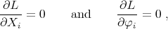
1.1. Statement of the problem. The Lagrangian formulation of mechanical systems has shown to be very useful in the presence of holonomic constraints. When this kind of constraints is involved, one may attempt to reduce the number of generalized coordinates, in order to deal with an effective Lagrangian with a lesser number of degrees of freedom.
In some occasions, a decrease in the number of generalized coordinates may not be convenient. As shown in many textbooks, through the use of Lagrange multiplier techniques, a system of equations of motion may be obtained for the holonomic case from an increased Lagrangian [Lan70, Mor00].
The case of a Lagrangian mechanical system subjected to non-holonomic constraints is much more subtle. General non-holonomic constraints have largely been discussed in articles [dLdD96, LM95] and textbooks [AKN93, Gol80, Lan70, LL76, NF72, Par62, Ros77, Run66], though only a restricted variety of cases has been considered in them. Very often works only deal with linear constraints; in other occasions they assume Chetaev's condition [CIdLdD04] or D'Alembert's one. It is probably worthwhile to remark that it is unfortunate that the above mentioned conditions are often referred to as principles, since this use might mislead the reader to consider them as some kind of fundamental law of nature; and the fact is that some systems do not satisfy these conditions, as shown in the example of section 3.
Instead, Hamilton's principle, also known as the principle of least action, is so fundamental that any physical theoretical framework can be based on it; for example classical mechanics, general relativity, the electroweak standard model, and quantum chromodynamics.
For many decades physicists knew the correct equations of motion for mechanical systems with general non-holonomic constraints; however, it is remarkable that no derivation of these equations from Hamilton's principle has been found in the literature. It has even been indicated that this derivation is not possible [Run66][SC70].
The equations of motion for systems subject to general non-holonomic constraints are derived in this work, starting from Hamilton's principle. This derivation makes use only of variational tools. The notation followed here has deliberately been chosen as close as possible to that of physics textbooks.
In this work we deal with a mechanical system, described by the Lagrangian
subject to the  , with
  , general non-holonomic constraints
|
| (1) |

which by assumption are considered independent. By independent it is meant that the Jacobian matrix  has rank
  .
.
1.2. Previous works. The subject of the derivation of the equations of motion for a mechanical system under the restriction of non-holonomic constraints has been studied for a long time. Derivations have normally been restricted to a subvariety of cases, and they usually use ad-hoc methods. For example in [Run66], in which the linear case is treated, the author recognizes: "... equation (5.10) is here accepted because of its empirical success. For the moment it should simply be regarded as a result which is known to be correct."
In particular, in relation to the question whether it is possible to derive the equations of motion from Hamilton's principle, Rund writes [Run66]: "... there exists a voluminous and rather confusing literature on the subject ...". And his answer to the question is that "the principle of Hamilton (as defined in the present context) is applicable to a dynamical system subject to constraints if and only if these constraints are holonomic." We will show in this article that his answer is not correct; we present a derivation from Hamilton's principle in the case of non-holonomic constraints.
One of the references Rund might had had in mind was probably the textbook by Pars [Par62], which treats the non-holonomic linear problem in section 8.16 and states: "We may be tempted to expect that a theorem analogous to Hamilton's principle may hold in the class  of curves satisfying the equations of constraints, i.e. we may expect
  to be stationary (the end-points in space and time being fixed) in the class
  . It comes as something of a shock to discover that this is not true." In fact, this assertion is misleading. For Pars, the class
  represents the set of trajectories that satisfy the constraints. So his assertion implies his expectancy that the variations involved in Hamilton's principle must be in the class
  ; but this is what characterizes the so called ‘Lagrange problem'; and it is known that it does not describe mechanical systems with non-holonomic constraints.
There are recent articles in which the nonholonomic dynamics is studied. In particular in [CdLdDM03] it is stated that: "In the nonlinear case, there does not seem to exist a general consensus concerning the correct principle to adopt. The most widely used model is based on Chetaev's principle, which will also be adopted in the present paper."
The correct equations of motion for mechanical systems with nonholonomic constraints have been known for many years. However the techniques involved in the justifications for them has varied. For example, it is attributed to Appell [App11] [Ray72] the deduction of the equations of motion from a generalization of Gauss's principle of least constraints.
We think it is worthwhile to point out that the source of some confussion in the problem of determination of equations of motion for mechanical systems subject to constraints, is that the method of subjecting the variations to the constraints, in the holonomic case, does work and allows us to obtain the correct equations of motion. This has induced the community [NF72] to think that the same method should be applied to the nonholonomic case. But it is known that this does not work. In what follows we show that allowing for general variations is the correct technique to derive the equations of motion for both cases, holonomic and nonholonomic.
We can see that the derivation of the equations of motion for nonholonomic dynamics has been an open problem and our contribution intends to settle this issue.
2.1. The Lagrange multipliers in the case of functions. Before treating the problem of the variational principle of Lagrangian mechanics in the presence of non-holonomic constraints, it is convenient to recall the use of Lagrange multipliers when applied to the case of extreme of functions.
Let us consider the case in which one would like to find a critical point of a function  subject to the conditions
|
| (2) |
and
|
| (3) |

Thinking of the variables  as coordinates of the space
  , we know that the gradients of functions are orthogonal to the surfaces on which these functions are constant. Therefore, the previous conditions imply that for any vector
  tangent to the surfaces determined by (2) and (3), one must have
|
| (4) |

and
|
| (5) |

where  represents the gradient operator and
  denotes the natural contraction
 between 1-forms and vectors [KN63]. Also, at a point
  in which
  has a critical point, one should have
|
| (6) |

Then if  and
and  at
at  , the set of vectors
  compatible with the constraints, i.e., satisfying (4) and (5), form an
  -dimensional subspace of the tangent space at
  . All vectors in this subspace must also satisfy (6). Therefore, one infers that there must exist constants
  and
and  such that
|
| (7) |

since otherwise the vectors satisfying (6) would lie outside of the  -dimensional subspace generated by the conditions (4) and (5). The constants
  and
and  are called the Lagrange multipliers of the problem.
The original problem is then transformed to find the solutions of (7) subject to (2) and (3).
For more constraints, this procedure generalizes in the obvious way.
2.2. The functional case. An interesting question is to see whether the ideas recalled above have an extension to the case of functionals.
In the study of Hamilton's principle, the analog to equation (6) is given by
|
| (8) |
![( ∫t2 ) ∫t2 r [ ( ) ] ( ) ∑ ∂L- d- ∂L- δ Ldt = ∂qi - dt ∂q˙i δqi dt = 0, t1 t1 i=1](/img/revistas/ruma/v47n2/2a1245x.png)
where the displaced trajectory  is given in terms of the variations
  by
by 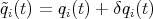 and which are subject to the boundary conditions

In equation (8) the analog of the vector  introduced in (4)-(6) is determined by the ‘components'
  , that is

while the analog of the covector  is determined by
|
| (11) |
where it is noted that  is minus the Lagrangian derivative
 ![[L]](/img/revistas/ruma/v47n2/2a1256x.png) as defined in [AKN93]; while
as defined in [AKN93]; while  is a vector in the tangent space
  of the configuration space
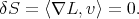
  [AKN93]. Finally, the natural product between the covector and vector is determined by the integration,
|
| (12) |
![t t ∫ 2 ∫ 2∑r [ ∂L d ( ∂L )] ⟨∇L, v⟩ ≡ ∇L ⋅ v(t) dt = --- - -- --- δqi dt, t t i=1 ∂qi dt ∂ ˙qi 1 1](/img/revistas/ruma/v47n2/2a1260x.png)
where the operator  is used to denote summation over the components of the covector
  and those of the vector
  .
.
The product  denotes the natural contraction between one forms and tangent vectors of the set of paths
  [AKN93] that have a definite initial point at
  and final point at
  in
in  . If
. If  is a path in the space
  , then a vector in the tangent space of
  at the point
  consists of a smooth vector field
  on
on  along the path
  such that
  and
and  . Such a vector
  is called a variation vector field [AKN93]; while the set
  can be considered as the components of a vector in the tangent space of the infinite dimensional manifold
  .
.
Then, defining the action  as
as
|
| (13) |
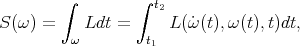
and using the above notation, one has from Hamilton's principle that
|
| (14) |
From now on we will continue using the standard notation  to denote the variations, instead of the more abstract
  notation.
Due to the existence of the constraints (1) it is clear that the variations  , for each individual generalized coordinate
  , can not be taken as linearly independent. In fact, let us assume that the trajectory
  satisfies the
  constraints (1). Then a variation of the constraints will give
|
| (15) |
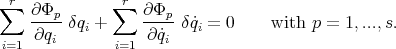
In order to obtain an expression that can be compared with (8) or (14), it is convenient to integrate this expression with respect to time, in the interval ![[t1,t2]](/img/revistas/ruma/v47n2/2a1291x.png) , from which one obtains
, from which one obtains
|
| (16) |
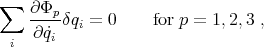
![∫ t2( ∑r ∑r ) ∫ t2∑r [ ( )] ∂Φp-δq + ∂Φp-δ˙q dt = ∂Φp- - -d ∂Φp- δq dt = 0. t1 ∂qi i ∂q˙i i t1 ∂qi dt ∂q˙i i i=1 i=1 i=1](/img/revistas/ruma/v47n2/2a1292x.png)
Therefore, using the above notation one has
|
| (17) |
These  equations are the analog to (4) and (5) in the previous section.
Following the logic as used in the case of functions, but now extended to infinite dimensional spaces, one deduces by analogy that there must exist scalars
  such that
This equation is the analog to equation (7); and we still may call the functions  Lagrange multipliers.
Therefore, one has
|
| (19) |
or explicitly
|
| (20) |
![t2 ( [ ( ) ] [ ( ) ]) ∫ ∑r ∂L d ∂L ∑s ∂Φp d ∂ Φp --- - -- --- + ηp(t) ----- -- ---- δqi dt = 0. t1 i=1 ∂qi dt ∂q˙i p=1 ∂qi dt ∂ ˙qi](/img/revistas/ruma/v47n2/2a12101x.png)
It is important to note that one can obtain a different expression involving the constraints by multiplying equations (15) by  and integrating with respect to time; namely
| (21) |
![( ) ∫ t2 ∑r ∂ Φ ∑r ∂Φ ηp ---pδqi + ---pδ˙qi dt = t1 i=1 ∂qi i=1 ∂ ˙qi ∫ t2 ∑r ( [ ( ) ] ) ηp ∂Φp-- d- ∂-Φp - ˙ηp∂-Φp δqi dt = 0. t1 i=1 ∂qi dt ∂ ˙qi ∂ ˙qi](/img/revistas/ruma/v47n2/2a12103x.png)
|
| (22) |
![∫t2 r ([ ( )] s ) ∑ ∂L- d- ∂L- ∑ ∂Φp- ∂qi - dt ∂ ˙qi + ˙ηp∂ ˙qi δqi dt = 0. t1 i=1 p=1](/img/revistas/ruma/v47n2/2a12104x.png)
Equations (20) and (22) are not completely equivalent; there are singular cases in which (20) can not be applied, but equation (22) has no problem. These cases are the ones that show critical points; namely cases in which  , for some
  . However, since a basic assumption of the problem is that the Jacobian of the system of equations (1) has rank
  , it is clear that equation (22) will not have any difficulties, even in the case of critical points. Therefore, equation (22) must be used.
It is very easy to think of cases in which this problem arises; as a simple example of a critical point, let us consider the single constraint  . Then one can easily see that although
  , the corresponding Jacobian has rank 1.
Defining  one can express (22) as
|
| (23) |
![∫t2 r ( [ ( )] s ) ∑ ∂L- d- ∂L- ∑ ∂Φp- ∂q - dt ∂ ˙q + λp ∂ ˙q δqi dt = 0. t1 i=1 i i p=1 i](/img/revistas/ruma/v47n2/2a12111x.png)
Any critical case can be thought of as the limiting case of a family of constraints which are not critical. It is clear that expression (23) has no difficulty in this limit, so that it can be used even in a critical case.
The rest of the analysis is the usual one; that is, let us choose the  functions
  in such a way that the equations
|
| (24) |
![[ ( ) ] ∑s ∂L-- d- ∂L- + λp (t)∂-Φp = 0, for i = 1, ...,s, ∂qi dt ∂ ˙qi p=1 ∂q˙i](/img/revistas/ruma/v47n2/2a12114x.png)
are satisfied. These constitute a system of  equations for the
  unknown functions
  .
.
In this way one is left with the equation
|
| (25) |
![∫t2 r ( [ ( ) ] s ) ∑ ∂L- d- ∂L- ∑ ∂Φp- ∂qi - dt ∂q˙i + λp ∂q˙i δqi dt = 0. t1 i=s+1 p=1](/img/revistas/ruma/v47n2/2a12118x.png)
From the assumption that the constraints are independent, one deduces that in principle it is possible to express  of its arguments in terms of the rest. So, if it is necessary, one could make a coordinate transformation to express the constraints in terms of
|
| (26) |

which constitute  differential equations for the
  functions
  with
with  , assuming that
  with
with  are given arbitrarily.
Therefore, in (25) one can take the variations 
 independently, which means that one must satisfy
|
| (27) |
![[ ( ) ] ∑s -∂L - d- ∂L- + λp ∂Φp-= 0, for i = s + 1,...,r. ∂qi dt ∂q˙i p=1 ∂q˙i](/img/revistas/ruma/v47n2/2a12129x.png)
From all this, one deduces that the functions  , which satisfy Hamilton's principle under the constraints, must satisfy the set of equations
|
| (28) |
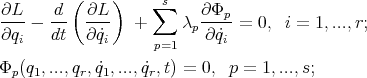
for the total set of functions
|
| (29) |

It should be clear from this presentation that the particular case of holonomic constraints must be treated from equation (20), since in this case, the assumption that the Jacobian, with respect to the arguments  , has rank
  , makes (20) a non-singular expression. Explictly one would have
|
| (30) |
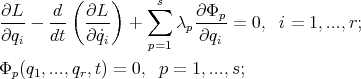
for the set of unknowns
|
| (31) |

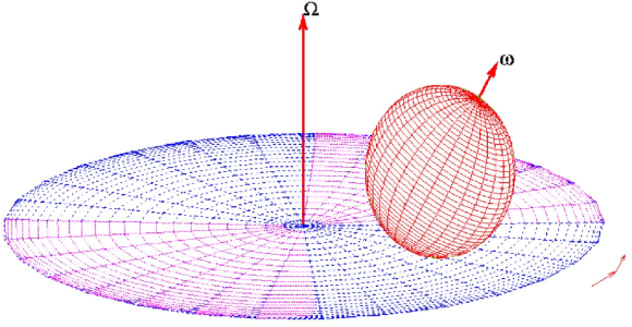
3. The classical problem of the rolling ball on a turntable
3.1. Example where Chetaev's condition fails. Consider a rigid ball of mass  and radius
  rolling on a uniformly rotating table with no sliding, as shown in figure 1. Here
  denotes the position of the center of the ball. We will choose a Cartesian coordinate system whose
  -axis will be perpendicular to the plane of the table and its upwards positive direction is characterized by the unit vector
  . The ball is assumed to be spherical and to have uniform mass density, so that its moment of inertia around an axis through its center of mass is
  .
.
The degrees of freedom in this problem can be described in terms of the infinitesimal movements. Let us denote with  an arbitrary small motion of the center of the ball, and with
  an arbitrary small rotation of it. Then the corresponding velocities are
  and
and  .
.
The contact condition in terms of the coordinate  of the center of the ball, the angular velocity
  of the rotating table (pointing upward) and that of the ball
  may be written as
|
| (32) |

where the symbol " " represents the vector product.
This constraint gives us an example in which the Chetaev's condition:
|
| (33) |
does not hold.
|
|
3.2. Newtonian approach. The Newtonian equations of motion are:
|
| (34) |

and
|
| (35) |
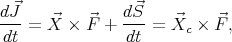
where  is the total force acting on the ball, due to the contact with the table,
  is the total angular momentum,
  is the intrinsic angular momentum and
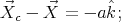
  denotes the point of contact between the ball and the turntable. It is easy to see that
|
| (36) |
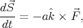
therefore, the equation of the intrinsic angular momentum is
|
| (37) |
where it is important to recall that in the case of an homogeneous sphere one has
|
| (38) |

Taking the time derivative of the constraint (32) one obtains
|
| (39) |
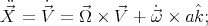
while from the angular momentum equation (37) one obtains
|
| (40) |
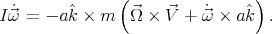
Now let us note that  , and
, and  , so that
|
| (41) |
Substituting into (39) and using the value of  it is obtained
|
| (42) |
or equivalently
|
| (43) |
whose solution describes a circular motion and  is a fixed point.
It should be observed that  and so
  is constant and undetermined.
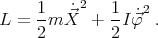
3.3. Lagrangian approach. The Lagrangian corresponding to this system is
|
| (44) |
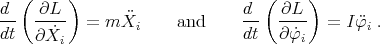
In order to obtain the equations of motion, it should be first noted that
|
| (45) |
whereas
|
| (46) |
Applying equations (28) to this system, one deduces
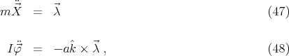
where in this case the  in equation (28) actually are the components of a vector
  . Multiplying this last equation by
  , and taking into account that
  is normal to
  , one has
|
| (49) |
Substituting this identity in (47), and making use of the constraint equation (32) to replace  , the following differential equation is obtained
|
| (50) |
which is equivalent to the Newtonian equation (42) deduced above and therefore shares the same space of solutions.
The equations of motion (28) are frequently mentioned in the literature; however, either they were not deduced from Hamilton's principle or their deduction did not consider the general case. For example equation (12) in the first chapter of reference [AKN93] is deduced assuming Chetaev's condition, although they do not refer to it.
In references [dLdD96, LM95, Gol80, Lan70, LL76, NF72, Par62, Ros77, Run66] the non-holonomic conditions are restricted to linear expressions in the velocities.
To our knowledge, ours is the first derivation of the equations of motion from Hamilton's principle for the general non-holonomic case.
We acknowledge support from CONICET and SeCyT-UNC. We have benefited from talks with H. Cendra and J. Solomin.
[AKN93] V.I. Arnold, V.V. Kozlov, and A.I. Neishtadt. Mathematical aspects of classical and celestial mechanics. In V.I. Arnold, editor, Dynamical Systems III. Springer-Verlag, 1993. [ Links ]
[App11] P. Appell. Sur les liasons exprimees par des relations non lineaires entre les vitesses. Comptes Rendus de lâAcadmie des Sciences Paris, 152 (1911), 1197-1199. [ Links ]
[CdLdDM03] J. Cortés, M. de León, D. Martín de Diego, and S. Martínez. Geometric description of vakonomic and nonholonomic diynamics. Comparison of solutions. SIAM J. Control Optim., 41:1389-1412, 2003. [ Links ]
[CIdLdD04] Hernán Cendra, Alberto Ibortl, Manuel de León, and David Martín de Diego. A generalization of Chetaev's principle for a class of higher order nonholonomic constraints. J.Math.Phys., 45:2785-2801, 2004. [ Links ]
[dLdD96] Manuel de León and David M. de Diego. On the geometry of non-holonomic lagrangian systems. J. Math. Phys., 37:3389-3414, 1996. [ Links ]
[Gol80] Herbert Goldstein. Classical mechanics. Addison-Wesley, Reading, Massachusetts, second edition, 1980. [ Links ]
[KN63] Shoshichi Kobayashi and Katsumi Nomizu. Foundations of Differential Geometry, volume I. John Wiley & Sons, 1963. [ Links ]
[Lan70] Cornelius Lanczos. The variational principles of mechanics. Dover Pub. Inc., Mineola, fourth edition, 1970. [ Links ]
[LL76] L.D. Landau and E.M. Lifshitz. Mechanics. Pergamon Press, Oxford, third edition, 1976. [ Links ]
[LM95] Andrew D. Lewis and Richard M. Murray. Variational principles for constrained systems: theory and experiment. Int. J. Nonlinear Mech., 30:793-815, 1995. [ Links ]
[Mor00] O.M. Moreschi. Fundamentos de la Mecánica de Sistemas de Partículas. Editorial Universidad Nacional de Córdoba, Córdoba, 2000. [ Links ]
[NF72] Ju. I. Neǐmark and N.A. Fufaev. Dynamics of nonholonomic systems. In Translations of Mathematical Monographs, volume 33. American Mathematical Society, 1972. [ Links ]
[Par62] L.A. Pars. An introduction to the Calculus of Variations. Heinemann, London, 1962. [ Links ]
[Ray72] John R. Ray. Nonholonomic constraints and Gauss's principle of least constraint. Am.J.Phys., 40:179-183, 1972. [ Links ]
[Ros77] Reinhardt M. Rosenberg. Analytical Dynamics of Discrete Systems. Plenum Press, New York, 1977. [ Links ]
[Run66] Hanno Rund. The Hamilton-Jacobi theory in the calculus of variations. D. van Nostrand Co. Ltd., London, 1966. [ Links ]
[SC70] Eugene J. Saletan and A.H. Cromer. A variational principle for nonholonomic systems. Am.J.Phys., 38:892-897, 1970. [ Links ]
Osvaldo M. Moreschi
FaMAF, Universidad Nacional de Córdoba
Ciudad Universitaria,
(5000) Córdoba, Argentina.
moreschi@fis.uncor.edu
Gustavo Castellano
FaMAF, Universidad Nacional de Córdoba
Ciudad Universitaria,
(5000) Córdoba, Argentina.
Recibido: 29 de septiembre de 2005
Aceptado: 29 de agosto de 2006

