


Serviços Personalizados
Journal

Artigo
 Inglês (pdf)
 Artigo em XML
 Referências do artigo
 Enviar este artigo por email
Indicadores
-
 Citado por SciELO
Links relacionados
-
 Similares em
SciELO
Similares em
SciELO
Compartilhar

 Permalink
Revista de la Unión Matemática Argentina
versão impressa ISSN 0041-6932versão On-line ISSN 1669-9637
Rev. Unión Mat. Argent. v.48 n.1 Bahía Blanca jan./jun. 2007
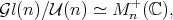
Non Positively Curved Metric in the Space of Positive Definite Infinite Matrices
Esteban Andruchow and Alejandro Varela
Abstract We introduce a Riemannian metric with non positive curvature in the (infinite dimensional) manifold  of positive invertible operators of a Hilbert space
  , which are scalar perturbations of Hilbert-Schmidt operators. The (minimal) geodesics and the geodesic distance are computed. It is shown that this metric, which is complete, generalizes the well known non positive metric for positive definite complex matrices. Moreover, these spaces of finite matrices are naturally imbedded in
  .
.
Key words and phrases. positive operator, Hilbert-Schmidt class
2000 Mathematics Subject Classification. 58B20, 47B10, 47B15
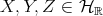
The space  of positive definite (invertible) matrices is a differentiable manifold, in fact an open subset of the real euclidean space of hermitian matrices. Let
  be hermitian matrices and
  positive definite, the formula

endows  with a Riemannian metric, which makes it a non positively curved, complete symmetric space. This metric is natural: it is the Riemannian metric obtained by pushing the usual trace norm on matrices to
  by means of the identification
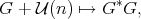
where  and
and  are, respectively, the linear and unitary groups of
  . This example has a universal property: every symmetric space of noncompact type can be realized isometrically as a complete totally geodesic submanifold of
  [7].
[7].
These facts are well known, have been used in a variety of contexts, and have motivated several extensions. For example, in the interpolation theory of Banach and Hilbert spaces [6], [16], in partial differential equations [15], and in mathematical physics [12], [17], [9]. They have also been generalized to infinite dimensions, i.e. Hilbert spaces and operator algebras: [17], [3], [2] [5], [1].
The purpose of this note is to introduce a Riemannian metric in the space  of infinite positive definite matrices, that is the set of positive and invertible operators on an infinite dimensional Hilbert space
  , which are of the form

where  and
and  , the class of Hilbert-Schmidt operators, i.e. elements
  such that
 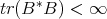 . We shall regard
  as an infinite dimensional manifold, in fact as an open subset of an apropriate infinite dimensional euclidean space, and introduce a Riemannian metric in
  , whichs looks formally identical to the metric for finite matrices. It will be shown that with this metric
  becomes a non positively curved, complete Riemannian manifold, which contains in a natural (isometric, flat) manner all spaces
  .
.
Therefore  can be regarded as a universal model, containing isometric and totally geodesic copies of all finite dimensional symmetric spaces of non compact type.
Let us fix some notation. We shall denote by  the usual norm of
  and by
  the Hilbert-Schmidt norm:
 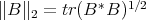 . Denote by

and

Note that since  is infinite dimensional, the scalars
  and the operators
  in
in  are linearly independent. In particular, one has that
  if and only if
  and
and  . Formally,
 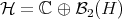 and
and 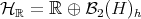 , where
  denotes the real Hilbert space of selfadjoint Hilbert-Schmidt operators. Let us define

Clearly this inner product makes  ,
,  , respectively, complex and real Hilbert spaces, where the scalars
  and the operators (in
  ) are orthogonal. The space
  will be considered with the relative topology induced by this inner product norm. It follows that the maps
  ,
,  and
and  ,
,  are orthogonal projections and their adjoints are the inclusions, which are therefore isometric.
Note that  means that
  and the spectrum of
  is a subset of
  . Indeed, the first assertion follows from the fact that
  , and the second is obvious.
In what follows, we denote by  the norm of
  . No confusion should arise with the norm of
  , because the former extends the latter.

Let us prove some elementary facts concerning the topology of  .
.
Proposition 2.1.  is open and convex in
  .
.
Proof. The fact that  is convex is apparent. Let
  . Since
  is positive and invertible, it follows that the eigenvalues of
  are bounded from below by
  , and do not aproach
  . Then there exists
  such that
  , or in other words,
  is positive and invertible. Consider the ball

We claim that if  , then
  . Indeed,
  . Then
  and the operator norm
  . Then
  and
and  , and therefore

which is positive and invertible. It follows that  . □
. □
The following elementary estimations will be useful.
 , then
Proof. Let  be the singular values of
  . Then
  . On the other hand,
  . Since the singular values accumulate eventually only at
  , clearly one has
  or
or  for some
  . In either case

which proves the first assertion. For the second,  . Since
  ,
,  . Then

By an argument similar to the one given above,  , and the second assertion follows. □
If  , one has the usual inequalities
  and
and  . As a consequence of 2.2, one has that the product
  is continuous, and therefore smooth, as a map from
  to
to  .
.
Next we show that the inversion map  ,
,  is smooth. The second inequality in 2.2, shows that
  can be renormed in order to become a Banach algebra. Indeed, putting
  , one obtains


is  .
.
Proof. The map  is the restriction of the inversion map of the regular group of the Banach algebra
  , which is an analytic map [14], to the smooth submanifold
  . □
. □
Note that in fact  is real analytic in
  (
( , being open in
  , has in fact real analytic structure).
We finish this section establishing certain identities which are satisfied by the inner product of  . Because it is defined in terms of the trace, this inner product inherits certain symmetries. But not others: for example, it is easy to see that if
  (selfadjoint) and
  , then
  may not be equal to
  .
.
Lemma 2.4. Let  and
and  , then the following hold:
 .
. .
.
Proof. The proof is a simple verification, and is left to the reader. The only issues here are the properties of the trace and the fact that scalars are orthogonal to operators in  . □
. □
3. NON POSITIVELY CURVED METRIC ON 
For  , consider the following inner product on
  (regarded as the tangent space
  ):
):
 | (3.1) |
First note that in fact it is a positive definite form, which varies smoothly with  , because the inversion map is smooth. Also note that it looks formally similar to the nonpositively curved metric for the space
  of positive definite finite matrices. However there are significant differences. For instance, if
  is finite dimensional, clearly
  is
is  (
( dimension of
  ), but the inner product defined on
  Is not the same as the trace inner product. An evidence of this is that in general
  for
for  ,
,  .
.
Nevertheless, the known formulas for the geodesics and curvature from the finite dimensional case, can be extended in this context. The reason for this is that the covariant derivative has the same formula as in the matrix case.
Proposition 3.1. The Riemannian connection of the metric defined in (3.1) is given by
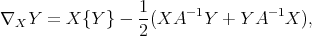 | (3.2) |
where  is a tangent vector at
  , and
, and  is a vector field. Here
  denotes derivation of the field
  in the
  direction, performed in the ambient space
  .
.
Proof. The formula (3.2) defines a connection in  . It clearly takes values in
  , which is the tangent space of
  at any point, and also verifies the formal identities of a connection. Also it is apparent that it is a symmetric connection. Therefore, in order to prove that it is the Riemannian connection of the metric from (3.1), it suffices to show that the connection and the metric are compatible. This amounts to proving that if
  is a smooth curve in
  and
and  are tangent vector fields along
  , then
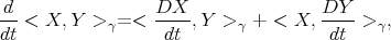
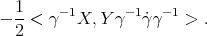
where as is usual notation,  . On one hand, using that
 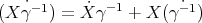 , and that
 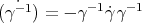 , one has
  | (3.3) |
On the other hand
   | (3.4) |
In the expression above, one may use the first identity in Lemma 2.4 to replace  by
by 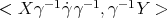 and
and  by
by 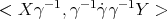 . Then proving the equality of (3.3) and (3.4) is equivalent to prove that

This is the same as the second identity in Lemma 2.4, with 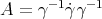 and
and  . □
. □
As a consequence, one obtains that the curvature tensor has the same expression as in the matrix case [3] [5]:
![R (X, Y )Z = - 1-A [[A -1X, A -1Y],A -1Z ], A 4](/img/revistas/ruma/v48n1/1a02178x.png) | (3.5) |
for  ,
,  . Here
 ![[ , ]](/img/revistas/ruma/v48n1/1a02181x.png) denotes the usual commutator for operators.
denotes the usual commutator for operators.
Theorem 3.2.  has non positive sectional curvature.
Proof. Compute
![< R (X, Y )Y,X > = - 1 < [[A -1X, A- 1Y],A -1Y ],XA -1 > A A 41 -1 - 1 2 -1 = - 4{< A-1 X (A-1 Y )- ,1XA ->1 - - 2 < A Y A XA Y,XA > + + < (A -1Y )2A -1X, XA -1 >}.](/img/revistas/ruma/v48n1/1a02183x.png)
Again we may use the same identity from Lemma 2.4 as follows:

The other terms above can be modified likewise. Let us denote 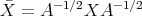 and
and 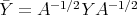 . Then
 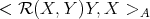 equals

Let us compare 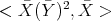 and
and  . Note that
  , let
, let  ,
,  . Then

Analogously

After cancellations, in order to compare  and
and  it suffices to compare
  and
and  . By the Cauchy-Schwarz inequality for the trace, one has
Therefore

Analogously one proves that

It follows that 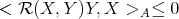 .
.
□
Remark 3.3. As was stated above, the fact that the formula to compute the Riemannian connection looks formally equal for  and for the space of positive definite finite matrices (in fact, also for positive invertible operators of an abstract
  -algebra [3], [5]) implies that one knows the explicit form of the geodesic curves. Let
  . Then the curve
 | (3.6) |
is a geodesic, which is defined for all  , and joins
  and
and  .
.
Then  is a simply connected (in fact convex) manifiold on non positive sectional curvature. It follows [10], [11] that the geodesic (3.6) is the unique geodesic joining
  and
and  . In fact one has the following:
Corollary 3.4. The curve given in (3.6) is the unique geodesic joining  and
and  , and it realizes the geodesic distance. The manifold
  is complete with the geodesic distance.
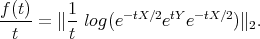
The geodesic distance of a non positively curved simply connected manifold has also the following property [10]: if  and
and  are two geodesics of
  , then the map

is convex. As in [5], we obtain the following consequence of this fact:
 and
and 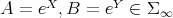 . Then
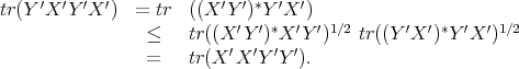
Proof. The proof follows as in Thm. 3 of [5]. We outline the argument. Let  and
and  . These are geodesics of
  which start at
  and verify
  and
and  . The function
  is convex, with
  . Then
  for
for ![t ∈ [0,1]](/img/revistas/ruma/v48n1/1a02233x.png) . Note that
. Note that  . Then
If  is small, then
 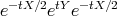 is close to
  , and therefore one has the usual power series for the logarithm,
  . Using also the power series of the involved exponentials and taking limit
  , one obtains

□
The map  provides a symmetry for
  . It is clearly a diffeomorphism with
  . Note that it is isometric. Indeed, if
  is a curve in
  with
with  and
and  , then
 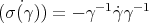 . Then
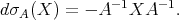
Then

which equals  by the first identity in Lemma 2.4.
 IN
IN  .
.Fix a positive integer  and let
  be an
be an  -dimensional subspace of
  . Let
. Let  be the orthogonal projection onto
  , and
, and  . The space
  of
of  positive definite (invertible) matrices identifies naturally with the space
  of positive invertible operators of
  . We shall consider the manifold
  with the Riemannian metric

This metric is well known in differential geometry ([15],[16]), and has been thoroughly studied and generalized to various infinite dimensional contexts ([3], [5]).
There is also a natural map from  into
into  ,
,

Note that  is well defined:
  has finite rank and therefore
  is a finite rank perturbation of the indentity.
Proposition 4.1. The map  is an isometric imbedding.
Proof. Clearly, it is injective. Let  and
and  be hermitian elements of
  , regarded as tangent vectors of
  at
at  . Apparently,
  . In particular, the range of
  is
is  which is complemented in
  . One has

Note that 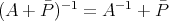 , where
  denotes the inverse of
  in
in  . Also
  , and then
 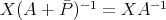 is a finite rank operator, in particular,
 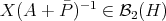 . Then

□
Remark 4.2. Another implication of the fact that the connections of  and
and  look formally identical, is that the maps
  are flat inclusions. The spaces
  regarded as submanifolds of
  , are not curved in
  . In particular these submanifolds are geodesically complete, or in other words, geodesics of
  are also geodesics of the ambient space
  . One may fix
  an orthonormal basis for
  , and consider
  the span of
  . Let
. Let  . Then via this family of imbeddings, one may think of
  as an ambient for all spaces
  of positive definite matrices, of all possible sizes.
[1] Corach, G., Maestripieri, A.L.; Differential and metrical structure of positive operators. Positivity 3 (1999), 297-315. [ Links ]
[2] Corach, G., Porta, H., Recht, L.A.; Splitting of the positive set of a C*-algebra, Indag. Mathem., N.S. 2 (4), 461-468. [ Links ]
[3] Corach, G., Porta, H., Recht, L.A.; The geometry of the space of selfadjoint invertible elements in a C*-algebra. Integral Equations Operator Theory 16 (1993), no. 3, 333-359. [ Links ]
[4] Corach, G., Porta, H., Recht, L.A.; Geodesic and operator means in the space of positive operators, International J. Math. 4 (1993), 193-202. [ Links ]
[5] Corach, G., Porta, H., Recht, L.A.; Convexity of the geodesic distance on spaces of positive operators. Illinois J. Math. 38 (1994), no. 1, 87-94. [ Links ]
[6] Donoghue, W.; The interpolation of quadratic norms, Acta Math. 118 (1967), 251-270. [ Links ]
[7] Eberlein, P.; Structure of manifolds of nonpositive curvature. Global differential geometry and global analysis 1984, Lecture Notes in Mathematics 1156, Springer, Berlin, 1985. [ Links ]
[8] Kobayashi, M., Nomizu, K.; Foundations of Differential Geometry, Interscience, New York, 1969. [ Links ]
[9] Kosaki, H.; Interpolation theory and the Wigner-Yanase-Dyson-Lieb concavity, Comm. Math. Phys. 87 (1982/83), 315-329. [ Links ]
[10] Lang, S.; Differential and Riemannian Manifolds, Springer, New York, 1995. [ Links ]
[11] McAlpin, J.; Infinite dimensional manifolds and Morse theory, Ph. D. thesis, Columbia University, 1965. [ Links ]
[12] Pusz, W., Woronowicz, S.L.; Functional calculus for sesquilinear forms and the purification map, Rep. Math. Phys. 8 (1975), 159-170. [ Links ]
[13] Raeburn, I.; The relationship between a commutative Banach algebra and its maximal ideal space J. Functional Analysis 25 (1977), no. 4, 366-390. [ Links ]
[14] Rickart, C.E.; General theory of Banach algebras , van Nostrand, New York, 1960. [ Links ]
[15] Rochberg, R.; Interpolation of Banach spaces and negatively curved vector bundles. Pacific J. Math. 110 (1984), no. 2, 355-376. [ Links ]
[16] Semmes, S.; Interpolation of Banach spaces, differential geometry and differential equations. Rev. Mat. Iberoamericana 4 (1988), no. 1, 155-176. [ Links ]
[17] Uhlmann, A.; Relative entropy and the Wigner-Yanase-Dyson-Lieb concavity in an interpolation theory, Comm. Math. Phys. 54 (1977), 21-32. [ Links ]
Esteban Andruchow
Instituto de Ciencias,
Universidad Nacional de Gral. Sarmiento,
J. M. Gutierrez 1150,
(1613),Los Polvorines, Argentina
eandruch@ungs.edu.ar
Alejandro Varela
Instituto de Ciencias,
Universidad Nacional de Gral. Sarmiento,
J. M. Gutierrez 1150,
(1613),Los Polvorines, Argentina
avarela@ungs.edu.ar
Recibido: 19 de mayo de 2005
Aceptado: 30 de noviembre de 2006

