Harmonic Functions on the closed cube: an application to Learning Theory

O.R. Faure, J. Nanclares, and U. Rapallini

 Presented by R. A. Macías

Abstract. A natural inference mechanism is presented: the Black Box problem is transformed into a Dirichlet problem on the closed cube. Then it is solved in closed polynomial form, together with a Mean-Value Theorem and a Maximum Principle. An algorithm for calculating the solution is suggested. A special feedforward neural net is deducted for each polynomial.

Key words and phrases. Dirichlet Problem, Diffusion Equation, Black Box, Convex Bodies

2000 Mathematics Subject Classification. 31-99, 52-99

1. Heuristic Introduction

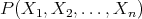
One of the main questions facing the field of Artificial Intelligence is the following input/output problem:

---

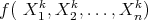
Given a finite number of instances or cases of a function as training data:

infer, relying only on the given training data, unknown cases or instances of , generalizing or predicting those yet unknown cases.

---

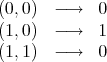
For example, we are given cases of a binary function:

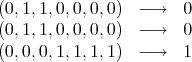
and we have to predict, say:

The problem may be restated as follows:

---

Given a binary function on a subset of the vertices of the th dimensional unit cube, infer its values on the rest of the vertices. We must find a way of extending the given data without introducing extra information.

---

The flow of heat is a powerful process for flattening boundary values, losing information until a steady state is reached with a final minimum of potential energy and a maximum of entropy (in short, with all possible flatness).

Thus we may say heuristically that the information of the whole domain with its boundary , the training data and the final harmonic function equals the information at the boundary when the process starts, the rest is a powerful flattening process ending in a function without local maxima or minima. Thus the process adds no information to the initial training data.

Consider the -dimensional temperature flow (heat equation):

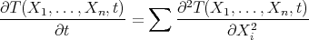such that on the vertices of the cube in a function 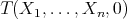is given as an initial temperature distribution. We only fix as given data at some vertices of the cube. If we let flow to the rest of the cube, always maintaining at the chosen vertices, and let  , once the steady sate (not equilibrium) is reached will take values on the whole cube and we may predict the values of on all the vertices. The limit function will be harmonic. The most important property of the solution is this: the potential equation solves the following variational problem:

In a given physical system find the function on the unit cube compatible with the given data and with minimum potential energy:

2. On the unit cube

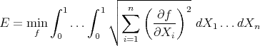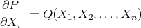
Definition 2.1. A P1P (Potential polynomial of degree 1 in each variable) will consist of a finite sum of monomials in the variables:

such that each (real valued) variable has at most degree 1; all the coefficients also are real-valued.

The most general P1P with real-valued coefficients will have the form:

where all the sums run over all the different sub-indices , and where no repeated sub-indices are allowed (there is no ). A special case is the purely boolean where the monomials are composed with variables or their boolean negations and the coefficients may be 0 or.

Every well formed formula in the predicate calculus has a logical equivalent in this disjuntive normal form. P1Ps:

are functions in the space : their derivatives

also are P1Ps, independent of , which implies that all second derivatives are zero, which makes P1Ps harmonic functions in .

Consider again the -dimensional heat equation:

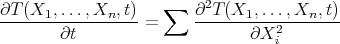On the vertices of the cube in a function is given as a fixed initial temperature distribution. Stepwise we may let it flow until the system converges to a steady state, keeping the initial data fixed, first to edges,once the edges attain a steady state which will be preserved, then to 2-dimensional facets, and so on until we have a temperature distribution on all the boundary such that it preserves the given data with un unceasing flow of heat at the initial vertices which preserves the initial information, and last allowing it to diffuse into the interior points of the -dimensional cube.

The resulting function when is the unique solution of Dirichlet's problem (see [1] and [4]): Keeping boundary data on some vertices fixed (it may be just 1 vertex) find in the whole cube the solution of Laplace's equation:

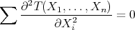This final steady state is not the state of equilibrium (see [9]). The flow of heat in order to sustain the boundary conditions keeps the system away from it.

We are given a finite number of instances or cases of a function on a subset of the vertices of the cube in , and we are required to find on all the cube and to express it as a P1P on the training data.

Let:

be boolean variables, identified with m vertices of the -dimensional cube, and let

the given values of as training data.

Call the convex hull of the vertices.

1. Assign to the edge of two linked vertices a P1P consistent with the values of on the linked vertices. That is, assign 0 or 1 or some or some to the actual edge, according to the training data.
2. Proceed in the same way with all the facets of , stepwise on each and all dimensions of the boundary of . In each case we are solving Laplace's equation with s on each boundary of each facet of .
3. When all the boundary of has been modelled, again solve Laplace's equation, this last time in dimensions, to get a unique harmonic function on , again a P1P in variables.
4. The expression of the P1P thus obtained is automatically extended with identical expression, to all the cube (in fact to all ). If we assume there is data on a few points  of the closed cube, then any continuous function defined at those points might grow to be a solution to Laplace's equation inside the cube (see [1]).

We get unicity through 'our' Dirichlet problem.

The following is our main result:

Theorem 2.1. There is only one solution  for our Dirichlet problem on the closed cube taking the values on its vertices, which is harmonic on each & all the facets of the cube.

Proof. The case is obvious. Consider a matrix of order  whose rows stand for the different vertices of the cube, and whose columns are:

We choose the first row or vertex to be , the case in which the variables are zero; and the first columnto be corresponding to 1. is a matrix of order . For example if we have is:

and is:

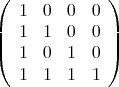We proceed to generate  : the columns are the previous ones plus the new ones:

We may write:

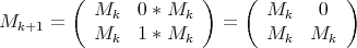An elementary excercise in algebra gives us the result:

By the induction hypothesis the determinant of is not zero, then the determinant of is not zero.

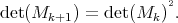
The linear equations:

for any given have exactly one solution; then:

is the unique solution to our Dirichlet problem on the closed -dimensional unit cube. □

3. Modelling P1P's

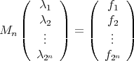
The potential energy of each function is calculated from the variational formula:

The following data are a modified form of a decision tree solving a 'tennis puzzle'(see [14], Chapter 2 ).

A Boolean function is defined in 13 examples:

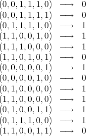
We proceed to calculate a least squares linear fit to the data; all the 2⁶ regressors are used. We find the P1P model:

as a fairly good representation of the function.

Warning:   Our solution does not always end in a minimum description length P1P. If we are given :

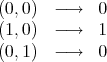
and we are asked to find the value corresponding to :

The flow of heat will give us the chosen solution:

with the following model

with potential energy equal to .

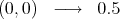
If instead we put:

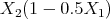
we get a potential energy equal to and a model given by But with:

we get a potential energy equal to and a model given by .

In other words: the solution model is the longest.

Again, given :

The flow of heat will give us:

with potential energy and model given by .

If we put:

we get a potential energy equal to and a model is

If we put :

the potential energy is equal 1.416 and the model is .

The first solution is chosen, and it is not the shortest one.

4. Neural Nets

Every P1P has an equivalent neural net: Each variable is an input neuron and the rest is an and/or scheme; the real coefficient of each monomial is the weight of the corresponding neuron. For example:

may be directly interpreted as a neural net and as a NeuPro code. Weights are set to 1 and the threshold to . The monomial will enter other neurons with a weight equal to its coefficient .

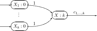
Figure 1. Monomial:

On the other hand all the monomial neurons will be connected to neuron with a threshold equal to .

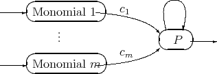
Figure 2.

The weight of each monomial is its coefficient in the P1P. Consider as example:

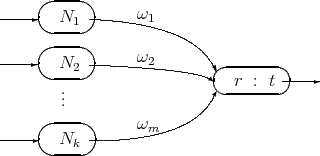
Figure 3.

It translates directly into the following NeuPro code (see [11]):

We started with an I/O situation from which we may infer the underlying function  expressing it as a P1P; then we obtain a 'natural' neural net representing and finally we translate mechanically the neural net into a NeuPro program.

5. Concluding Remarks

1. Assuming training data is given at a subset of the vertices of a unit cube we map the prediction problem into finding the solution of the heat equation in the whole cube.
2. Our inference machine is then the natural flow of temperature fixing the training data during the process in a typical Dissipative Structure. (See [9])
3. The unique limit solution as is harmonic which means it is the function with minimum potential energy compatible with the given data.
4. The solution also has maximum Boltzmann's entropy: where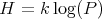 is the number of microstates (or complexions) in the actual physical final macrostate and is Boltzmann's constant.
5. The P1P solution has an inmediate translation into a neural net and into a Neupro (or Prolog) code.
6. We may translate Prolog code into P1P's obtaning a model of the code, a kind of 'self model'of the program. (See Appendix). This feature might be useful in the debugging process.
7. The P1P solution is often, but not always, a Minimum Description Length object.

6. Appendix

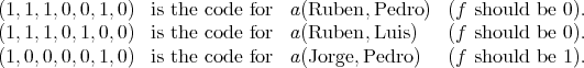
We map into our scheme a prolog program modelling the grandfather relation. Consider the program:

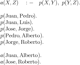
Its meaning: relation holds between objects and if () relation holds between objects and and () relation holds between and .

We may code this information as follows: We assign predicates and a with 1 and 0 respectively.

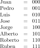
We code the predicates as follows :

We find, as a fitted model for the underlyng theory with an error = the following function:

Now we test this model for trying the following examples:

We run the model for and find :

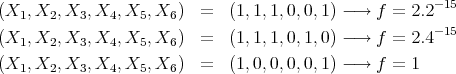
in almost perfect agreement with the theory.

References

[1]    Axler S., Bourdon P. & Ramey W. (2001) Harmonic Function Theory. Springer Verlag.        [ Links ]

[2]    Bundy A. (1983) The Computer Modelling of Mathematical Reasoning. Academic Press.        [ Links ]

[3]    Chaitin G. (1975) A theory of program size formally identical to Information Theory. Journal ACM Vol. 22 #3, 329-340.        [ Links ]

[4]    Courant R. & Hilbert D. (1953) Methods of Mathematical Physics. Interscience Publishers.        [ Links ]

[5]    Hand D., Mannila H. & Smyth P. (2001) Principles of Data Mining. MIT Press.        [ Links ]

[6]    Kelley J. (1955) General Topology. Van Nostrand University Series in Higher Mathematics.        [ Links ]

[7]    Kon M.A. & Plaskota L. (2000) Information Complexity of Neural Networks. Neural Networks.        [ Links ]

[8]    Mendelson E. (1964) Introduction to Mathematical Logic. Van Nostrand.        [ Links ]

[9]    Nicolis G. & Prigogine I. (1989) Exploring Complexity. Freeman & Co.        [ Links ]

[10]    Poggio T. & Girossi F. (1990) Regularization Algorithms for learning that are equivalent to multilayer Networks. Science # 247 pp. 978-982.        [ Links ]

[11]    Rapallini U. & Nanclares J. (2005) Intérprete NeuPro utilizando la NeuPro Abstract Machine. XI Congreso Argentino de Ciencias de la Computación. Concordia ER.        [ Links ]

[12]    Shannon C. (1949) A Mathematical Theory of Communication. University of Illinois Press.        [ Links ]

[13]    Sussman H. (1975) Semigroup Representations Bilinear Approximation of input/output maps and generalized inputs. Lecture Notes in Economics & Math. Systems. Mathematical Systems Theory 131, Springer Verlag.        [ Links ]

[14]    Mitchel T. (1997) Machine Learning. WCB McGraw Hill.        [ Links ]

[15]    Traub J.F. & Werschultz (1999) Complexity & Information. Cambridge University Press.        [ Links ]

O. R. Faure
Facultad Regional Concepción del Uruguay,
Universidad Tecnológica Nacional,
Ing. Pereira 676,
E3264BTD Concepción del Uruguay (ER), Argentina
ofaure@frcu.utn.edu.ar

J. Nanclares
Facultad Regional Concepción del Uruguay,
Universidad Tecnológica Nacional,
Ing. Pereira 676,
E3264BTD Concepción del Uruguay (ER), Argentina
nanclarj@frcu.utn.edu.ar

U. Rapallini
Facultad Regional Concepción del Uruguay,
Universidad Tecnológica Nacional,
Ing. Pereira 676,
E3264BTD Concepción del Uruguay (ER), Argentina
rapa@frcu.utn.edu.ar

Recibido: 2 de octubre de 2007
Aceptado: 22 de octubre de 2007