


Servicios Personalizados
Revista

Articulo
 Inglés (pdf)
 Articulo en XML
 Referencias del artículo
 Enviar articulo por email
Indicadores
-
 Citado por SciELO
Links relacionados
-
 Similares en
SciELO
Similares en
SciELO
Compartir

 Permalink
Revista de la Unión Matemática Argentina
versión impresa ISSN 0041-6932versión On-line ISSN 1669-9637
Rev. Unión Mat. Argent. v.48 n.3 Bahía Blanca 2007
Cluster categories and their relation to Cluster algebras, Semi-invariants and Homology of torsion free nilpotent groups
Gordana Todorov
Dedicated to María Inés Platzeck for her 60th birthday and Hector Merklen for his 70th birthday
Abstract. The structure of cluster categories [BMRRT] is well suited for the combinatorics of cluster algebras [FZ1] with the main correspondence being between tilting objects and clusters. Furthermore it was shown in [IOTW] that there is a close relation between domains of virtual semi-invariants and simplicial complexes associated to cluster categories. Also the same simplicial complexes associated to cluster categories are related to the Igusa-Orr pictures in the homology of nilpotent groups.
The purpose of this paper is to define and relate several, quite different notions, and therefore the paper is mostly a survey paper, including many results without proofs and also some indications about work in progress. With this in mind, the paper is divided in the following way.
In Section 1 we define and state main properties of cluster categories. The results are mostly from [BMRRT].
In Section 2, cluster algebras with no coefficients are defined (2.1) and several results about their relation to cluster categories are given . We consider only acyclic case; in (2.2) the main bijection theorem between cluster variables and indecomposable objects of the cluster category is stated; in (2.3) the denominators of nonpolynomial cluster variables are described in terms of dimension vectors of exceptional indecomposable representations; in (2.4) weak positivity condition of cluster variables is stated as a consequence of the quite technical proposition, and the proof of the bijection theorem is given. Also, Cluster determines seed conjecture is proved in 2.5.
Section 3 is mostly survey section, where we first recall definitions and theorems about classical semi-invariants, and then give definition and properties of virtual representation spaces and virtual semi-invariants. We only state the main theorems and for proofs refer to [IOTW].
Finally, Section 4 contains a short summary of the results about homology of nilpotent groups and the relation to the simplicial complex of tilting object in the corresponding cluster category.
1.1. A motivation. The categories of finitely generated modules over hereditary artin algebras, together with their derived categories, are very well understood. Since there were clear indications (e.g.[FZ1]) that there was close relation between the indecomposable modules and cluster variables of the cluster algebras, at least in the finite representation type, via root systems, it was quite natural to study and develop the theory of certain orbit categories of the derived categories which perfectly reflect the combinatorics of cluster algebras.
1.2. Derived category. We recall the standard definitions and notation: Let  be a quiver with
  vertices and no oriented cycles and
  a field. Then
  , the associated path algebra is hereditary. Let
  be the category of finitely generated
  -modules, and
  the derived category of bounded complexes in mod
 . Since
  is hereditary the derived category is easy to describe: the objects in
  are finite direct sums of the objects in
 ![∪ {(mod Λ [i])} i](/img/revistas/ruma/v48n3/3a0210x.png) and the morphisams in
and the morphisams in  can be described in the following way:
 for
for  in
in  ,
,
![1 HomDb (M, N [1]) = Ext Λ(M, N )](/img/revistas/ruma/v48n3/3a0215x.png) for
for  in
in  ,
,
![HomDb (M, N [i]) = 0](/img/revistas/ruma/v48n3/3a0218x.png) for
for  in
in  and all
![HomDb (X [i],Y[i]) = HomDb (X, Y )](/img/revistas/ruma/v48n3/3a0222x.png) for
for  in
in  and all
  .
.
1.3. Cluster category. In order to define the corresponding cluster category, we consider the endofunctor: ![-1 - 1 b b F = τ [1] = [1]τ : D → D ,](/img/revistas/ruma/v48n3/3a0226x.png) where
where ![b b [1] : D → D](/img/revistas/ruma/v48n3/3a0227x.png) is the suspension functor, and
is the suspension functor, and  is the Auslander-Reiten functor. Then, the cluster category
  is defined to be the orbit category, i.e. the objects in
  are
are  -orbits, and the morphisams in
  are
are  , where
  and
and  are
are  -orbits of
  and
and  .
.
From the above definition it is easy to see that a set of representatives of the orbits may be chosen in ![add(ind Λ ∪ {Pi[1]}ni=1)](/img/revistas/ruma/v48n3/3a0239x.png) . Often we will use the same symbol for the objects in
. Often we will use the same symbol for the objects in  and their orbits in
  .
.
1.4. An example. Let  be the Dynkin diagram of type
  with the following orientation and labeling of the vertices:
  . Let
. Let  be the non isomorphic simple
  representations, or simple
  -modules, let
  be the nonisomorphic indecomposable projective
  representations (
 -modules), and let
  be the nonisomorphic indecomposable injective
  representations (
 -modules). Consider the Auslander-Reiten quiver of mod
 and
and  :
:
![S3[- 1] P3 P1 [1 ] S2 [1] S3[1] P3[2] \\ // \\ // P2 I2 P2[1] I2[1] P2 [2] // \\ // \\ // P1 S2 S3 P3 [1] P1[2] S2[2]](/img/revistas/ruma/v48n3/3a0256x.png)
A set of representatives for the  -orbits may be chosen to be the following 9 objects:
 ![{P1,P2, P3,S2,I2,S3, P1[1 ],P2 [1],P3[1]}.](/img/revistas/ruma/v48n3/3a0258x.png)
1.5. Tilting objects. Tilting objects are defined in a similar way as tilting modules. First we define ![∐ ∐ Ext1C ( ˜X, ˜Y ) := iExt1Db(X, F iY ) = iHomDb (X, F iY [1]) Λ](/img/revistas/ruma/v48n3/3a0259x.png) . Then, we define
. Then, we define  to be an exceptional object in
  if
if  . Define a tilting object (basic) to be a maximal exceptional object in
  without multiplicities. As stated in 1.3 we will usually use the same symbol for the objects in
  and their orbits in
  .
.
1.6. Tilting seeds. The notion of tilting seed is introduced for the sake of setting up a good correspondence between "cluster category" terminology and "cluster algebra" terminology, in order to be able to write rigorous proofs. A tilting seed is defined to be a pair  , where
  is a basic tilting object and
  is the quiver of
  . Notice that the tilting object
  determines the quiver
  .
.
1.7. Exchange pairs. The following theorems give precise conditions when an indecomposable summand of a tilting object can be replaced by another indecomposable object, i.e. they "can be exchanged".
Theorem 1.7.1. [BMRRT] Let  be a basic tilting object with
  indecomposable. Then, there exists exactly one object
  not isomorphic to
  , such that
  is also a basic tilting object.
Definition 1.7.2. Using the notation from Theorem 1.7.1 we call the indecomposable objects  and
and  an exchange pair with respect to
  (or
(or  ).
).
Theorem 1.7.3. [BMRRT] Two exceptional indecomposable objects  and
and  form an exchange pair if and only if
  , where
  and
and  .
.
1.8. Tilting objects in the cluster category for  . We will use the same example and the same notation as in 1.4. In the following figure the vertices are labeled by representatives of indecomposable objects in the cluster category. Vertices are connected by a line segment if there are no extensions between the two corresponding objects. Consequently, each small triangle defines a tilting object and all tilting objects are given that way. There are 14 tilting objects in this example, e.g.
  ,
,  ,
, ![∐ ∐ (S1 [1] S2 P3 [1])](/img/revistas/ruma/v48n3/3a0289x.png) ,
, ![∐ ∐ (S1[1] P2[1] P3 [1])](/img/revistas/ruma/v48n3/3a0290x.png) etc.
etc.
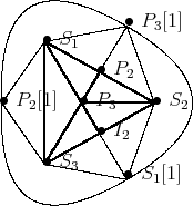
Figure 1. Tilting objects in the cluster category of 
1.9. Tilting mutations. Throughout the paper we will use 3 different ways to express the situation from the Theorem 1.7.1:
- Tilting mutation of an indecomposable object
 is
is  , with respect to
  :
:  e.g.
e.g.  with respect to the tilting object
 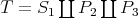 .
. - Tilting mutation of the tilting object
 at
at  is
is 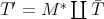 :
:  e.g.
e.g.  .
. - Tilting mutation of the tilting seed
 at
at  is the new seed
  :
: 
e.g.
 , with the extra information that
 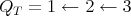 and
and  .
.
All examples refer to the cluster category in 1.8.
1.10. A construction of exchange pairs, i.e. tilting mutation. This construction uses the notion of minimal right approximation by a subcategory. Let  be a tilting object, where
  is an indecomposable summand. Let
  be a minimal right
  -approximation of
  . This approximation exists, since
  is additively generated by a finitely generated module
  . Let
. Let
 .
. 1.11. Some facts about exchange pairs. Here we state some of the facts (without proofs) and draw the commutative diagrams from [BMRRT].
 is indecomposable and exceptional,
 is a minimal left
  - approximation of
  ,
, ,
, and
and  form an exchange pair with respect to
  (or
(or  ).
).- Consider the AR-triangle for
 :
: 
![∐ | Kh Lh[- 1] | ----- M * --- AM * --τ-1M * ----- =| | | g f h ----- M * -----B ----- M| ------ g′ ′ B| ′ f τ- 1M *[1 ] = F M * ~=CΛ M *.](/img/revistas/ruma/v48n3/3a02131x.png)
 ,
,![∐ ∐ B ′ = Coker (h) Ker (h)[1] := Lh Kh [1]](/img/revistas/ruma/v48n3/3a02133x.png) ,
, is an isomorphism if and only if
  ,
, if and only if
  is AR triangle if and only if
  .
.- The vertical maps
 and
and  are left and right
  -approximations of
  and
and  (respec).
 - By considering AR triangle for
 we get a similar commutative diagram.
2. Cluster Algebras and Cluster Categories
In this section we want to indicate what correspondences exist between the categorical notions of cluster categories and combinatorial notions of cluster algebras.
Cluster algebras were defined by Fomin and Zelevinsky, in general with coefficients, however cluster categories are set to deal only with the cluster algebras without coefficients, so we will recall the definition of cluster algebras only in that case. We also point out that the "sign skew symmetrizable square matrices" correspond to valued quivers, with valuations on arrows being precisely the integer values of the entries of the corresponding matrix.
2.1. Cluster algebras; Definitions.
Cluster algebra  is a subalgebra of the field of rational functions
  , which is generated as algebra by cluster variables; cluster variables are defined to be all rational functions which appear in a certain collection of transcendence bases, called clusters; clusters are transcendence bases in
  which are obtained from an initial cluster after applying sequences of "cluster mutations" in every possible direction, but according to the rules prescribed by the matrices
  , (or equivalently, quivers
  ) as we will describe in 2.1.1.
We point out that at every stage of cluster mutations, there is a new pair formed  , called a cluster seed, where
  is the new cluster and
  is the new quiver. Initial cluster seed is a pair
  , where
  is a transcendence basis, called initial cluster and
  is the initial quiver (a matrix
  ).
).
Definition 2.1.1. Using the notation from above we now define cluster mutations (again, the same mutation expressed in 3 ways as in 1.9):
- Cluster mutation of
 with respect to the cluster seed
  is the new cluster variable
  obtained as
  .
. Notation
 .
. - Cluster mutation of the cluster
 at
at  is a new cluster
Notation:

- Cluster mutation of the cluster seed
 at
at  is the new cluster seed
  .
. Notation:
 , where
  new quiver obtained in quite a complicated way (see [FZ1]).
In general, this process of creating new cluster variables will never stop, however there is a precise classification of cluster algebras which have only finitely many cluster variables, as stated in the following theorem.
Theorem 2.1.2. [FZ2] A cluster algebra has finitely many cluster varibles, if and only if a Dynkin diagram appears as one of the quivers in the mutation process.
Starting with a fixed quiver  (no oriented cycles), one obtains a cluster algebra
  , with all of its notions: cluster seeds, clusters, cluster variables, cluster mutations. From the same quiver one can construct cluster category
  , with the tilting seeds, tilting object, indecomposable objects and tilting mutations. The following table contains main "cluster algebra" and "cluster category" notions, NOT as a theorem, but just to indicate where the correspondences should be. However, the theorems are stated afterwards.
 quiver
  -cluster algebra -cluster algebra | -- |  -cluster category, where -cluster category, where  |
 -initial cluster seed -initial cluster seed | -- | ![∐ ∐ (P1 [1 ] ⋅⋅ ⋅ Pn [1],Q )](/img/revistas/ruma/v48n3/3a02180x.png) -initial tilting seed -initial tilting seed |
 -any cluster seed -any cluster seed | -- |  -any tilting seed -any tilting seed |
 -any cluster -any cluster | -- |  -any basic tilting object -any basic tilting object |
 -any cluster variable -any cluster variable | -- |  -any indecomposable exceptional object -any indecomposable exceptional object |
Theorem 2.2.1. [FZ1], [MRZ] Suppose  is a Dynkin diagram. Then there exists a one-to-one correspondence
 cluster variables
 isoclasses of indecomposable objects
  .
.
Theorem 2.2.2. [BMRRT] Suppose  is a simply laced Dynkin diagram. Then there exist one to one correspondences (the second one being induced by the first):
 cluster variables
 isoclasses of indecomposable objects
 ,
,
{clusters} {basic tilting objects}.
It was conjectured in the same paper that similar one-to-one correspondences exist between cluster variables and exceptional indecomposable objects for all simply laced diagrams with no oriented cycles. The proof of this follows from the existence of two particular surjective maps, which are inverse bijections:
 ,
,
 .
.
The map  is the Caldero-Chapoton map from [CK2], and the existence of map
  is given in the following theorem.
Theorem 2.2.3. [BMRT] Let  be simply laced diagram with no oriented cycles.
(a) There exist well defined maps:
 cluster variables
 isoclasses of indecomp. exceptional objects},
 clusters
 tilting objects},
 cluster seeds
 tilting seeds}.
(b) All three maps:  are onto.
We will indicate main steps of the proof of the above theorem, since they include several other interesting results about the denominators of the cluster variables 2.3.4, weak positivity condition 2.4.6 and proof of the Fomin-Zelevinsky conjecture that cluster determines the entire cluster seed after cluster mutations 2.5.1.
Theorem 2.2.4. Bijection ([CK2],[BMRT]) Let  be simply laced diagram with no oriented cycles. Then there exist a bijection between cluster variables and exceptional indecomposable objects, inducing a bijection between clusters and tilting objects.
An illustration on  . We illustrate the above correspondence by using the same Figure 1 as we did for the objects, tilting objects and exchange pairs of the cluster category, but label the vertices now by the corresponding cluster variables.
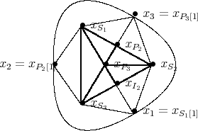
Figure 2. Clusters in the cluster algebra of 
- Vertices are labeled by cluster variables and cluster variables are labeled by the corresponding representatives of indecomposable objects in the cluster category.
- Vertices are connected by a line if the compatibility degree between the cluster variables is 0 which corresponds to no extensions between the corresponding two objects.
- Each small triangle defines a cluster and a basic tilting object.
- All clusters and all tilting objects are given that way.
- There are 14 clusters and 14 basic tilting objects in this example.
- The initial cluster
 is chosen in such a way, that the denominators of all other cluster variables are given by the dimension vectors of the corresponding
  -modules (see theorems in next section).
2.3. Denominators of cluster variables.
From this section, we only need notation, and the famous "Laurent phenomenon" theorem of Fomin and Zelevinsky. However we will also state known results about the monomials which appear in the denominators of the cluster variables.
Theorem 2.3.1. [FZ1] (Laurent phenomenon) The denominators of all cluster variables, when expressed in terms of the initial cluster, and then reduced, are monomials.
Notation: Let  be a monomial in variables
  . Denote the exponent vector by
  .
.
Theorem 2.3.2. [FZ1] Let  be a Dynkin diagram with alternating orientation. For each cluster variable in reduced form
  , there is an indecomposable module
  , such that
Theorem 2.3.3. [CCS2] Let  be any Dynkin diagram. For each cluster variable in reduced form
  , there is an indecomposable module
  , such that
  (Also [RT] and [CK1] have the same result.)
Theorem 2.3.4. [BMRT] Let  be any finite simply laced diagram with no oriented cycles. For each cluster variable in reduced form
  , there is an indecomposable exceptional module
  , such that
Proof. This follows from 2.4.6. □
2.4. Weak Positivity Condition and Conditions ( ,
,  ,
,  ).
).
These are essential notions for the proofs of the existence of the maps  ,
,  ,
,  , i.e. that the objects
  ,
,  ,
,  satisfy the desired conditions:
  is an indecomposable exceptional object,
  is a tilting object and
  is a tilting seed.
Definition 2.4.1. A polynomial  in variables
  is said to satisfy the weak positivity condition if
  for all
  , where
  is at the
  -th place.
Remark: If  satisfies the weak positivity condition, then
  does not have any non-constant monomial factors.
Definition 2.4.2. Let  be an initial cluster for a cluster algebra given by a quiver
  . A cluster variable
  is said to satisfy
  if:
if:
- either
 or
or  , where
  is a polynomial in
  and it satisfies positivity condition and
 - if
 , then there exists an indecomposable exceptional
  -module
  , such that
  .
.
Definition 2.4.3. If a cluster variable  satisfies condition (
 ), we (can) define:
![{ M if x = f∕m and ε(m ) = dimM α(x) := Pi[1 ] if x = fxi.](/img/revistas/ruma/v48n3/3a02269x.png)
Remark: We want to define  on all cluster variables. So far, we defined only on cluster variables satisfying (
 ). So, we will prove that ALL cluster variables satisfy condition (
 ) if the cluster algebra is acyclic with no coefficients.
This will be proved after the Proposition 2.4.4 and Corollary 2.4.6, however the proof involves clusters and cluster seeds as well. The corresponding conditions on clusters and cluster seeds will be denoted by: ( ),(
),( ) and we define them now.
Properties: ( ), (
), ( ), (
), ( ) Definitions and properties.
( ) is a property of a cluster variable
  consisting of two parts:
 or
or  , where
  satisfies positivity condition, and
 , for some indecomposable exceptional module
  .
. Notice: If
 satisfies (
 ), then
  is defined (i.e. it is an indecomposable exceptional object)(as in 2.4.2 and 2.4.3).
( ) is a property of a cluster
  consisting of two parts:
- each cluster variable
 satisfies (
 ), and
  is a tilting object.
 Notice: If
 satisfies (
 ), then
  can be defined as
 , which is a tilting object.
( ) is a property of a cluster seed
  consisting of two parts:
- the cluster
 satisfies (
 ), and
  .
. Notice: If
 satisfies (
 ), then
  can be defined as
 which is a tilting seed.
Proposition 2.4.4. Let  be a cluster seed satisfying (
 ). Consider a cluster mutation. Then:
-
 :
:- The new cluster variable satisfies (
 ).
).  :
:- The new cluster satisfies (
 ).
).  :
:- The new cluster seed satisfies (
 ).
).
-
 :
: commutes with mutations, i.e.
  .
. :
: commutes with mutations, i.e.
  .
. :
: commutes with mutations, i.e.
  .
.
Proof. We need to set up a bit more detailed and precise notation.
Let  be a cluster seed, where
  is a cluster.
Let  be a cluster mutation at
  .
.
Since  satisfies (
 ), there exists an object
  such that
  .
.
Denote  by
by  .
.
Let  be the new cluster variable defined via cluster mutation
  .
.
Then 
 .
.
Proof of a: WTS  satisfies (
 ). Let
  .
.
It is a tilting object since  satisfies (
 ).
).
Consider tilting mutation of  at
at  , i.e. exchange
  with another object
  .
.
Then  is the new tilting object.
Let  and
and  be the exchange triangles.
Notation and results from ([BMR2], 6.2) imply:
 if
if  and
and  .
.
At this point we brake the proof into several parts, depending on whether the representatives of  and
and  are modules or shifted projectives.
Case I: Both  and
and  are modules.
- Step 1:
 is an exact sequence of modules.
- Step 2:
- Describe
 , i.e. representatives of the summands of
  in the fundamental domain add(ind
![n Λ ∪ {Pi [1]}i=1)](/img/revistas/ruma/v48n3/3a02365x.png) . Consider the following commutative diagram, together with the AR-triangles as mentioned at the beginning:
. Consider the following commutative diagram, together with the AR-triangles as mentioned at the beginning: ![∐ | Kh Lh [- 1] | | | | 0 | | // ∐ -1 */ Kg Lg[- 1 ] τ M | // | | AM * h 0 | / | | // ---- * /--- ----- /---- 0 M | B| M| 0 / // | // | 0 g | A τM | | // | ′ ∐ τM| B = Kh [1] Lh / // | | 0 | | | | τ- 1M *[1] = F M *](/img/revistas/ruma/v48n3/3a02366x.png)
 implies
  and
and 
![∐ ∐ τ-1(Kg Lg[- 1])[1] ~= b (Kh [1] Lh) D](/img/revistas/ruma/v48n3/3a02370x.png)
Let
 with
with  injective and
  with no injective summands.
Let
 with
with  projective and
  with no projective summands.
![∐ ∐ ∐ ∐ τ-1Kg [1] τ- 1I τ-1Z ~=Db (Lh P [1] Y [1])](/img/revistas/ruma/v48n3/3a02377x.png)
By comparing shifts of nonprojectives, shifts of projectives and actual modules, get the following isomorphisms in the derived category:
![-1 ~ τ Kg [1]=Db (Y [1])](/img/revistas/ruma/v48n3/3a02378x.png) ,
, ![-1 ~ P (SocI )[1] = τ I =Db P[1]](/img/revistas/ruma/v48n3/3a02379x.png) ,
, 
![τ-1Kg [1] ~= (Y [1]) Db](/img/revistas/ruma/v48n3/3a02381x.png) implies
implies ![F Kg ~= (Y [1]) Db](/img/revistas/ruma/v48n3/3a02382x.png) and so
and so ![~ Kg =C (Y [1])](/img/revistas/ruma/v48n3/3a02383x.png)
Finally:
![′ ~ ∐ ∐ B =C (Lh Kg P [1])](/img/revistas/ruma/v48n3/3a02384x.png)
- Step 3:
- All
 ,
,  ,
,  satisfy condition (
 ) by assumption.
  ,
,  ,
,  ,
,  ,
,![xP[1] = (c(P∕rP )fP [1])](/img/revistas/ruma/v48n3/3a02393x.png) where
where 
 ,
,  ,
,  ,
,  ,
, ![fP [1]](/img/revistas/ruma/v48n3/3a02399x.png) satisfy positivity condition
satisfy positivity condition ,
,  ,
,  ,
,  .
. - Step 4:
 or
or  Reason:
- Step 5:
- Compute

![(f +f ⋅f ⋅m′⋅c ⋅f )(1∕f ) (xM )* = (xB(+xxMB)′)-= --B--Kg-Lh-(mB-(∕Pm∕rMP))-P[1]---M-](/img/revistas/ruma/v48n3/3a02408x.png)
- Step 6:
 satisfies condition (
 ). Reason:
  divides the rest of the numerator (Laurent phenomenon).
Numerator is a polynomial which satisfies positivity condition.
Numerator does not have any non-constant monomial factors.
Denominator is monomial
 , with
 is an indecomposable exceptional module.
- Step 7:
 This is exactly the statement that
  commutes with mutations, i.e. 2)a of the proposition.
Case II:  is not a module, i.e.
 ![M = P [1]](/img/revistas/ruma/v48n3/3a02418x.png) .
.
First, we point out that in this case  must be a module, since
  . We will just set up the exchange triangles and commutative diagrams, and the rest is similar kind of analysis, but somewhat more complicated.
![M = P [1]](/img/revistas/ruma/v48n3/3a02421x.png) implies that
implies that ![∐ B = C P ′[1]](/img/revistas/ruma/v48n3/3a02422x.png) , with
, with  non-projective and
  projective.
![M *[1 ] ~= P ∕P ′[1]](/img/revistas/ruma/v48n3/3a02425x.png) since
since ![dim Hom (M, M *[1]) = 1](/img/revistas/ruma/v48n3/3a02426x.png)
![| | | | | | | | | | // | / / ′ -1 ′ B | τ (P|∕P ) | // | | / | | AP∕P′ |h / | // | | / / ′/ ∐ ′ / ′ P ------P ∕P -- C P [1] -- P [1 ]-- (P ∕P )[1] // | | // | / / | | / | g | AI | | // | |/ / | I B ′ // | | / / | | / | | | | | | | τ- 1(P ∕P ′)[1] = F(P ∕P ′)](/img/revistas/ruma/v48n3/3a02427x.png)
Case III:  a module,
 ![* M = P [1 ]](/img/revistas/ruma/v48n3/3a02429x.png) . Similar to the previous case.
. Similar to the previous case.
This finishes the proof of  the new cluster variable
  satisfies condition (
 ) and also
  .
.
Proof of  The new cluster
  satisfies (
 ).
).
- Each cluster variable
 satisfies (
 ) condition by assumption and part
  .
.  is a tilting object.
Proof of  The new cluster seed
  satisfies (
 ).
).
- The new cluster
 satisfies (
 ) by
) by  .
. - The quiver of
 is equal to
  by [BMR].
This finishes the proof of the proposition. □
Corollary 2.4.5. Let  be a cluster seed satisfying condition (
 ). Let
  be a cluster mutation and
  the corresponding tilting mutation. Then:
  .
.
Corollary 2.4.6. Every cluster seed satisfies ( ), every cluster satisfies (
 ) and every cluster variable satisfies (
 ). In particular, every cluster variable is either of the form
  or
or  , for some weakly positive polynomial
  .
.
Proof. The initial seed  satisfies (
 ) condition. Since every cluster seed can be reached by a finite number of cluster mutations, and by the proposition every cluster seed at each step satisfies (
 ) condition it follows that all cluster seeds satisfy (
 ) condition. □
Proof. of the Theorem 2.2.3 : By the above corollary it follows that everything satisfies appropriate (
 ), (
), ( ), (
), ( ), and by the comments in the definitions of (
 ), (
), ( ), (
), ( ), all three maps (
 ), (
), ( ), (
), ( ) are defined. □
Proof. of the Theorem 2.2.3 : We will show that
  is onto. Let
  be a tilting seed. There exists a finite number of tilting mutations from the initial tilting seed to
  . Consider the same sequence of cluster mutations from the initial cluster seed. Use Corollary 2.4.5. □
2.5. Fomin-Zelevinsky Conjecture: Cluster Determines Seed.
The following was conjectured by Fomin and Zelevinsky (for any cluster algebra) and we prove it for the acyclic case with no coefficients.
Theorem 2.5.1 (BMRT). Let  and
and  be cluster seeds for an acyclic cluster algebra with no coefficients. Then
  .
.
Proof.  and
and  are tilting seeds. But,
  since tilting seed is determined by its tilting object. □
3. Semi-invariants and Cluster Categories
We first recall the definition and some of the classical theorems about semi-invariants, as done by Kac, Schofield, Derksen-Weyman for non-negative integral vectors. After that we state theorems for "mixed signs" integral vectors as done in [IOTW]. In particular, in the Dynkin diagram case, we state the relation between the simplicial complex of the partial tilting objects and the domains of semi-invariants .
3.1. Definitions; Representations and Semi-invariants. Let  be a simply laced quiver, where
  denotes the set of the vertices of
  , and
, and  is the set of the arrows of
  . Assume
  has no oriented cycles. Let
  be an algebraically closed field. Let
  be the number of the vertices in
  .
.
3.2. Representation space for  . The representation space for a non-negative integral vector
  is the affine space:
 will be called based representations with dimension vector
  . Every element of
  can be viewed as a collection of
  -matrices, one for each arrow
 . The group:
 , by
, by  . We use the convention that
  is the trivial group.
 3.3. Euler bilinear form. The vertices of the quiver are partially ordered by  if there is a directed path from
  to
to  and we choose a fixed extension of this partial ordering to a total ordering. The Euler matrix
  is defined as
  matrix with rows and columns labeled by
  (written in the order described above), with the diagonal entries equal to 1 and the entry
  (the number of arrows from
  to
to  ) for
) for  . The matrix
  gives a nonsymmetric bilinear form
 , which we call the Euler form.
 3.4. Some useful facts about the Euler form and Euler matrix.
 , i.e.
  for all representations
  and
and  such that
  and
and  .
.- The row of
 corresponding to the vertex
  , consists of coefficients of indecomposable projectives in the expression of
  .
.  gives coefficient vector of
  in terms of
  s.
s. always has non-negative coefficients, e.g. if
  then
then  .
.
3.5. Notation. Let  . We denote by
  the following projective representation:
  . Notice that
  .
.
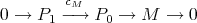
3.6. Canonical projective presentations. Recall, the canonical projective presentation of a representation  , with
  is:
is:
 and
and  . The mapping
  sends
sends  to
to  by the negative inclusion map; so, the generator of each
  maps to -(the image in
  of the generator of the corresponding
  ) and
) and  sends
sends  to
to  by the mapping
  induced by the arrow
  .
. Remark 3.6.1. The representation  can also be described as:
 and
and  .
.
3.7. Classical results on semi-invariants of quivers.
We recall now the notion of semi-invariants of a group acting on a variety and state the classical results about semi-invariants on the representation spaces of quivers by Kac, Schofield and Derksen-Weyman.
3.8. Definition of semi-invariants. For an algebraic group  acting on a variety
  , an element
  of the coordinate ring of
  is called a semi-invariant, if there exists a character
  of
of  such that for all
  and all
  :
:
3.9. Semi-invariants of quivers,  . The group
  acts on the representation space
  (see 3.2). Since the group
  is the product of general linear groups, the character
  is the product
  . The integral vector
  is called the weight of the semi-invariant. Note that if
  then
then  is indeterminate.
3.10. Fundamental theorems for semi-invariants of quivers. The First fundamental theorem (FFT) states that all semi-invariants of quivers are generated by determinants, the Saturation theorem describes all nonnegative vectors with semi-invariants of a given weight and the third theorem describes Generic decomposition of any non-negative integral vector  .
.
Theorem 3.10.1 (FFT,[S, DW1]). Let  be a quiver and
  . Then the ring of semi-invariants on
  is generated by
  , where

 , and representations
  satisfy
  . Furthermore, the weight of the semi-invariant
  is
is  .
. Remark 3.10.2. The condition  is equivalent to saying that the matrix of
  is square.
Definition 3.10.3. Let  . The support of
  is defined as

Theorem 3.10.4 (Saturation,[DW]). Let  . Then:

 where
where  means that the general representation of dimension
  has a subrepresentation of dimension
  .
. Before stating the generic decomposition theorem, recall the following definition: for  ,
,

 is algebraically closed). Since
  is upper semicontinuous this minimum is attained for generic modules of these dimensions. So, this definition agrees with the usual definition, i.e.
  , where
  are generic representations with
  and
and  .
. Theorem 3.10.5 (Generic decomposition,[K]). Any  has a unique decomposition of the form
  where
where  for all
  and each
  is a Schur root. Furthermore, general representation
  with
with  decomposes as
  with
with  where
where  are indecomposable representations which do not extend each other.
3.11. Virtual representation spaces and Virtual semi-invariants.
In this section we deal with integral vectors (not necessarily non-negative), define non-canonical generalized representation spaces and the virtual representation space as the direct limit of those. Similarly, we define semi-invariants on the generalized representation spaces and virtual semi-invariant as the induced map on the virtual representation space.
3.12. Projective decomposition of integral vectors. Let  and let
  with
with  . We refer to
  as a projective decomposition of
  . Note that there is a unique minimal projective decomposition where
  have disjoint supports.
3.13. Generalized representation spaces for integral vectors. Let  . For each projective decomposition
  of
of  , a non-canonical generalized representation space is defined as

3.14. Stabilization maps. Given any  we have the stabilization map:
  which sends
  to
to

3.15. Virtual representation spaces for integral vectors. Let  . Then all representation spaces
  form a directed system with the above stabilization maps. We define the virtual representation space as the direct limit:
3.16. Semi-invariants on Generalized representation spaces. The space
 is an affine space with the natural action of the group
  which is given by
  for each
  . (We point out that this is a different action then in 3.2).
Since  is an affine space its coordinate ring is a polynomial ring, hence polynomial semi-invariants are defined as in 3.8.
3.17. Virtual semi-invariants. A virtual semi-invariant on  is a function
  induced by a family of semi-invariants
  on the representation spaces
  , which are compatible with stabilization maps (3.14).
3.18. Characters . Notice that for  , each element of
  can be written as an
  upper triangular matrix
  with
with  and diagonal entries
  The reason is that the vertices are partially ordered by
  if there is a directed path from
  to
to  and this partial ordering is extended to a total ordering to write the matrix.
Remark 3.18.1. Given a projective representation  then any rational character of the group
  is of the form:
  with the vector
  ; and
; and  for polynomial characters. As before,
  is indeterminate if
  .
.
Remark 3.18.2. (a) A polynomial SI on  is a polynomial function
  so that:
  for some character
  , all
, all  and all
  .
.
(b) Furthermore  , with
  and
and  characters of
  and
and  respectively, and therefore of the form
  and
and  for
for  .
.
3.19. Weights of semi-invariants. If  are sincere (nonzero at every vertex) then
  above, call it
  . The well-defined
  is called the weight of the SI
  . Since the collection of
  for sincere pairs
  is cofinal in the directed system, the weights are well defined for virtual SI and have non-negative coordinates.
3.20. A construction of semi-invariants for  . We show that the determinants also give generalized SI and induce virtual SI.
Proposition 3.20.1. Let  be a projective decomposition of
  . Let
. Let  be a representation with
  . Then:
- The function
 is a polynomial SI on the generalized representation space
  ,
, - Weight(
 )=
)=  .
. - Furthermore,
 is compatible with stabilizations.
 - The induced semi-invariant
 on the virtual representation space
  has also weight equal to
  .
.
Definition 3.20.2. The support of  is defined to be the set of all
  so that
  on
on  for some projective decomposition
Theorem 3.20.3. (Virtual Saturation Theorem) The support of  is equal to

 is the general representation of dimension
  .
. Theorem 3.20.4. (Virtual Generic Decomposition) Any  has a unique decomposition of the form

 for all
  ,
,- Each
 is either a Schur root in degree
  or negative indecomposable projective in degree 1.
3.21. The finite case - Dynkin diagrams.
We show that the simplicial complex of the clusters can be identified with the domains of the generalized semi-invariants, which will also be identified with the Igusa-Orr pictures for the sets of simple roots [IO].
3.21.1. Simplicial complex of exceptional (or partial tilting) objects. The simplicial complex of the Dynkin diagram is defined to be the simplicial complex  , with vertex set

Theorem 3.21.1. (Simplicial complex and domains of semi-invariants theorem) [IOTW]. Let  be a Dynkin diagram of type
  . Then:
- The simplicial complex of the exceptional objects is homeomorphic to the
 sphere.
 - The image of the
 skeleton of
  in
in  is the union:
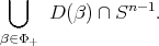
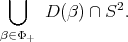
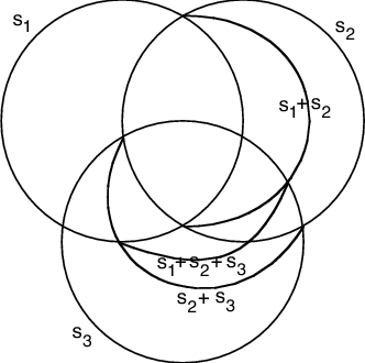
3.21.2. Illustration on the example of  . The image of the
  skeleton of
  in
in  is the union:
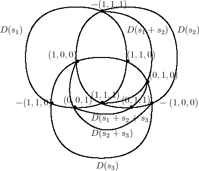
- The quiver is
 with Euler matrix
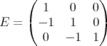
- Circles and semicircles, labeled by
 , denote the domains of semiinvariants (with weight
  ).
). - Vertices are labeled by the positive roots
 and negative projective roots.
 - Positive roots can also be viewed as dimension vectors of indecomposable representations by Gabriel's theorem, e.g.
 .
. - For example:
 has semi-invariants of weights
  and
and  .
. - For example:
 ,
,  ,
,  ,
, ,
,  all have semi-invariants of weights
  since
since  making
  iff
iff  .
. - The semiinvariant
 on a representation
is
 . This is only well-defined if coordinates
  are chosen. If these are changed by
  then
then  becomes
So, this semiinvariant has weight
 .
. - In the case
 we have
  . So,
. So,  does not contain points
  where
where  . So,
. So,  contains no points inside the
  circle.
 - Furthermore, any integral vector belongs to one of the simplices, and the generic decomposition is given in terms of the vertices of that simplex.
4. Homology of Nilpotent, Torsion-free Groups
4.1. Homology of groups and Lie algebras.
4.1.1. Homology of a group. The homology of a group  is defined by
More explicitly, we need to choose a free  resolution
  of
of  . Then
  is the homology of the complex
  . One standard complex is given by the bar resolution where
  is the free
  module generated by
  and the boundary map
  is given by

 is torsion-free, nilpotent, there is a smaller chain complex in which
  is generated by the set of all
  -element subsets of the nilpotent basis
  of
of  , see 4.2.7. There are various descriptions of this complex ([CP1], [IO]). One of the objectives of this work is to give a new canonical description of this smaller complex using root systems and semi-invariants in the case when
  is a monomial group (including groups of Dynkin type).
 4.1.2. Homology of a group - topological definition. We recall, but will not use that the homology of the group  is defined topologically by
  where
where  is the classifying space of the discrete group
  , also known as the Eilenberg-MacLane space
  .
.
4.1.3. Rational homology of a group. The rational homology of a group  is
is  .
.
4.1.4. Homology of a Lie algebra. The homology of a Lie algebra  ,
,  , is defined to be the homology of its Koszul complex
  given by
  with boundary
  given by
![∑ d(x ∧ ⋅⋅⋅∧ x ) = (- 1)i+j[x ,x ]∧ x ∧ ⋅⋅⋅∧ ^x ∧ ⋅⋅⋅∧ x^ ∧ ⋅⋅⋅∧ x 1 k i j 1 i j k i<j](/img/revistas/ruma/v48n3/3a02797x.png)
4.1.5. Rational homology of a Lie algebra. The rational homology of a Lie algebra  is
is  .
.
4.1.6. Lie algebra  associated to a group
  . To every group
  there is an associated graded Lie algebra
  given by
  with Lie bracket
![[ , ] : Li(G ) ⊗ Lj(G ) → Li+j(G )](/img/revistas/ruma/v48n3/3a02805x.png)
given by the commutator: ![[gGi+1,hGj+1 ] := [g,h ]Gi+j+1](/img/revistas/ruma/v48n3/3a02806x.png) .
.
4.2. Torsion-free Nilpotent groups.
4.2.1. Definition of Torsion-free, Nilpotent groups. Let  be a group and
  the chain of subgroups defined as
 ![Gi+1 = [G, Gi]](/img/revistas/ruma/v48n3/3a02809x.png) , where
, where ![[ , ]](/img/revistas/ruma/v48n3/3a02810x.png) denotes the group commutator operation, i.e.
denotes the group commutator operation, i.e. ![-1 -1 [g,h] = ghg h](/img/revistas/ruma/v48n3/3a02811x.png) for all
for all  . The group
  is said to be:
- Torsion free if
 is finitely generated free abelian group for all
  .
.  if there exists an
  such that
  .
.
Theorem 4.2.1 (Nomizu). [N54] The rational homology of a torsion-free nilpotent group  is isomorphic to the homology of the Lie algebra
  .
.
4.2.3. Remark. Nomizu [N54] gave the first example of a nilpotent torsion free group whose integral homology is not isomorphic to that of the associated Lie algebra. Dwyer [D] points out that the upper triangular matrix group (the nilpotent group associated to the Dynkin diagram  ) has
) has  -torsion in its homology for all
  . The rational homology is given by the following theorem of Bott and Kostant.
Theorem 4.2.2. [Bo][Ko] The rank of the  -th homology of the nilpotent subalgebra of a semisimple Lie algebra spanned by the positive roots is equal to the number of elements of the Weyl group of weight
  . For example, the rank of
  is equal to the number of elements
  of the symmetric group on
  letters for which there are
  pairs
pairs  with
with  .
.
4.2.4. Koszul complex. The Koszul complex gives both the integral and rational homology for any Lie algebra  and in particular for the Lie algebra
  and therefore, by Nomizu's theorem, it gives the rational homology of
  as well.
4.2.5. Cenkl and Porter. In [CP1] they give an algorithm for constructing the integral cochain complex for the integral cohomology of  . (The integral cohomology determines the integral homology.) In [CP1] they construct a nilpotent torsion free group with a prescribed Lie algebra (the reverse of the usual construction).
4.2.6. A motivation from topology. Kent Orr proved that all Milnor  -invariants of links are represented by elements of
  of the fundamental group of the complement of the link. Igusa and Orr proved that
  has no torsion for nilpotent torsion free groups, using a particular complex in which boundaries are given by "pictures".
4.2.7. Remark. Each nilpotent torsion free group has a finite basis  which can be obtained as the union of preimages of the bases of the free abelian groups
  for
for  . These elements form a basis in the sense that every element in the group can be expressed uniquely in the form
  where
where  are integers.
- Let
 be preimages of a set of basis elements of
  .
. - Then
 is a minimal set of generators for the group
  , call these elements simple generators.
 - The number
 does not depend on the choice of the basis.
4.2.8. Igusa-Orr complex and "pictures". This is a particular ![ℤ [G ]](/img/revistas/ruma/v48n3/3a02854x.png) resolution of
resolution of  , which we will not describe precisely, but the following are some of the important facts about it:
 is freely generated by the sets of k-element subsets of the basis
  .
.- The boundary
 is recursively defined for each subset of
  .
. - Boundary is Koszul boundary plus additional terms.
- Boundary for each subset of
 corresponds to a "picture", i.e. a cell decomposition of sphere, satisfying certain necessary and sufficient conditions.
 - Left and right commutators in the group give the most efficient "collecting process".
- Different forms of commutators. The standard form of commutator is the left commutator
 , the original Igusa-Orr pictures use the right commutator
  , and for the Cluster-Semiinvarian pictures it is more convenient to use the middle commutator
  .
.
4.3.1. Definition of Monomial groups. These are special torsion free monomial groups, for which Igusa-Orr pictures are related to the Cluster-Semi-invariant pictures. A group  is called
  if it is:
- Torsion free,
- Nilpotent and
- There exists a basis
 satisfying:
 - a:
![[bi,bj] ⊂ B ∪ B -1 ∪ [1]](/img/revistas/ruma/v48n3/3a02873x.png)
- b:
- For any three elements at least two commute
- c:
- For any
 ,
, ![[bi,bj]](/img/revistas/ruma/v48n3/3a02875x.png) commutes with both
commutes with both  and
and 
4.3.2. Maximal monomial groups. These will be monomial groups which are maximal in the following sense (but we need to point out a few facts):
- The number of elements in
 is an invariant of the group G.
 - Monomial groups with
 simple generators, for a fixed
  , are partially ordered by epimorphisms of groups, which send simple generators to simple generators (or their inverse).
 - Maximal elements with respect to this partial order are called Maximal monomial groups.
4.3.3. Dynkin diagrams and Maximal monomial groups. To each simply laced Dynkin diagram  with the set of positive roots
  , we associate a group
  defined by:
- Generators:
 and
and - Relations:
![{ [Θ (α),Θ (β)] = Θ(α + β )ε(α,β)](/img/revistas/ruma/v48n3/3a02890x.png) where
where  if
if  and
and  otherwise
 . Here
  denotes the Euler form.
We have the following facts, questions (and work in progress):
- Simply laced Dynkin diagrams define maximal monomial groups.
- Are all maximal monomial groups given by simply laced Dynkin diagrams (A,D,E) as above?
- Description of the groups (with appropriate modifications of the condition (3)), which will correspond to the other Dynkin diagrams (B,C,F,G).
4.4.1. An  example of Igusa-Orr picture.
- Circles and semicircles are labeled by positive roots
 for the Dynkin diagram
  . Any positive root
  is expressed as a sum of simple roots
- For the middle-commutator I-O picture the same labels are used for the elements of the associated nilpotent group
 , i.e. any positive root
  actually stands for
  , see 4.3.3.
 - A free
 resolution of
  is given by
  free module generated by subsets of
  with
with  elements, and with boundary given by the pictures.
 - The following picture describes the boundary
 as:
as: 
- Each term in the sum corresponds to a vertex, and is obtained by "reading" the picture.
- Circles and semicircles are labeled by positive roots
 for the Dynkin diagram
  . Labeling agrees with the same labeling of the same picture by the domains of semiinvariants.
4.4.2. I-O vs C-SI pictures. The original, right commutator Igusa-Orr and Cluster-Semiinvariant pictures are given below for the example of Dynkin diagram  .
.
- I-O picture has 12 tri-angles, 1 quadr-angle, 1 bi-angle
- C-SI picture is a simplicial complex, triangulation of a shpere with 14 tri-angles.
I-O 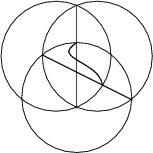 C-SI C-SI 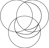 |
- Igusa-Orr pictures are Koszul boundary plus higher terms.
- Cluster-Semiinvariant pictures are modified Koszul boundary plus higher terms.
- Cluster-Semiinvariant pictures are more natural - simplicial complex.
- Plan to re-do Igusa-Orr algorithm to construct all Cluster-Semiinvariant pictures.
- Cluster-Semiinvariant pictures give the middle commutator Igusa-Orr pictures for the particular subset consisting of the simple generators
 of the group
  , which actually correspond to the set of simple roots in
  .
. - We believe that Cluster-Semiinvariant pictures can be used to construct, in a functorial way, all middle-commutator I-O pictures (for all subsets of
 .
.
This work was presented at:
CIMPA - UNESCO - ARGENTINA
Homological methods and representations of non-commutative algebras.
Mar del Plata,
Argentina
March 6 - 17, 2006
[Bo] Bott, Raoul, Homogeneous vector bundles, Ann. of Math. (2), 66, (1957), 203-248. [ Links ]
[BMR1] Buan A., Marsh R., Reiten I. Cluster-tilted algebras, preprint (2004) math.RT/0402075, to appear in Trans. Amer. Math. Soc. [ Links ]
[BMR2] Buan A., Marsh R., Reiten I. Cluster mutation via quiver representations, preprint (2004) math.RT/0412077 [ Links ]
[BMRT] Buan A., Marsh R., Reiten I., Todorov G. , preprint math.RT/, to appear in .(2004) [ Links ]
[BMRRT] Buan A., Marsh R., Reineke M., Reiten I., Todorov G. Tilting theory and cluster combinatorics, preprint math.RT/0402054, to appear in Adv. Math. (2004) [ Links ]
[CC] Caldero P., Chapoton F. Cluster algebras from cluster categories, preprint math.RT/0410187, (2004) [ Links ]
[CCS1] Caldero P., Chapoton F., Schiffler R., Quivers with relations arising from clusters ( case)., Preprint arxiv:math.RT/0401316, January 2004, to appear in Trans. Amer. Math. Soc. [ Links ]
[CCS2] Caldero P., Chapoton F., Schiffler R., Quivers with relations and cluster tilted algebras. Preprint arxiv:math.RT/0411238, November 2004. [ Links ]
[CK1] Caldero P., Keller B. From triangulated categories to cluster algebras, preprint math.RT/0506018, (2005) [ Links ]
[CK2] Caldero P., Keller B. From triangulated categories to cluster algebras II, preprint math.RT/0510251, (2005) [ Links ]
[CP1] Bohumil Cenkl and Richard Porter, Algorithm for the computation of the cohomology of I-groups, Algebraic topology (San Feliu de Guíxols, 1990), Lecture Notes in Math., vol. 1509, Springer, Berlin, 1992, pp. 79-94. [ Links ]
[CP2] Bohumil Cenkl and Richard Porter, Nilmanifolds and associated Lie algebras over the integers, Pacific J. Math. 193 (2000), no. 1, 5-29. [ Links ]
[D] W. G. Dwyer, Homology of integral upper-triangular matrices, Proc. Amer. Math. Soc. 94 (1985), no. 3, 523-528. [ Links ]
[DW1] Harm Derksen and Jerzy Weyman, Semi-invariants of quivers and saturation for Littlewood-Richardson coefficients. J. Amer. Math. Soc. 13 467-479 (2000). [ Links ]
[DW] Harm Derksen and Jerzy Weyman, On the canonical decomposition of quiver representations, Compositio Math. 133 (2002), no. 3, 245-265. [ Links ]
[FZ1] Fomin S., Zelevinsky A. Cluster Algebras I: Foundations, J. Amer. Math. Soc. 15, no. 2, 497-529 (2002) [ Links ]
[FZ2] Fomin S., Zelevinsky A. Cluster Algebras II: Finite type classification. Invent. Math. 154 (2003), no. 1, 63-121. [ Links ]
[FZ3] Fomin S., Zelevinsky A. Cluster Algebras III: Upper bounds and double Bruhat cells. Duke Math J. 126 (2005), No. 1, 1-52. [ Links ]
[IO] Kiyoshi Igusa and Kent E. Orr, Links, pictures and the homology of nilpotent groups, Topology 40 (2001), no. 6, 1125-1166. [ Links ]
[K] V. G. Kac, Infinite root systems, representations of graphs and invariant theory, Invent. Math. 56 (1980), no. 1, 57-92. [ Links ]
[Ko] Kostant, Bertram, Lie algebra cohomology and the generalized Borel-Weil theorem, Ann. of Math. (2), 74,(1961), 329-387. [ Links ]
[Kel] Keller B. On triangulated orbit categories, preprint, math.RT/0503240, (2005) [ Links ]
[Ker] Kerner O. ??? [ Links ]
[MRZ] Marsh R., Reineke M., Zelevinsky A. Generalized associahedra via quiver representations, Trans. Amer. Math. Soc. 355, no.10,4171-4186 (2003). [ Links ]
[N54] Nomizu, Katsumi . On the cohomology of compact homogeneous spaces of nilpotent Lie groups, Ann. of Math. (2) 59 (1954), 531-538. [ Links ]
[RT] Reiten I., Todorov G. Unpublished [ Links ]
[S] Aidan Schofield, Semi-invariants of quivers, J. London Math. Soc. (2) 43 (1991), no. 3, 385-395. [ Links ]
Gordana Todorov
Northeastern University
Department of Mathematics
360 Huntington Avenue
Boston, MA 02115, USA
todorov@neu.edu
Recibido: 1 de marzo de 2007
Aceptado: 27 de noviembre de 2007

