


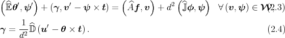
Servicios Personalizados
Revista

Articulo
 Inglés (pdf)
 Articulo en XML
 Referencias del artículo
 Enviar articulo por email
Indicadores
-
 Citado por SciELO
Links relacionados
-
 Similares en
SciELO
Similares en
SciELO
Compartir

 Permalink
Revista de la Unión Matemática Argentina
versión impresa ISSN 0041-6932versión On-line ISSN 1669-9637
Rev. Unión Mat. Argent. v.49 n.1 Bahía Blanca ene./jun. 2008
Finite element approximation of the vibration problem for a Timoshenko curved rod
E. Hernández*, E. Otárola†, R. Rodríguez‡, and F. Sanhueza§
* Partially supported by FONDECYT grant 1070276 and USM grant 12.05.26.
† Partially supported by USM grant 12.05.26.
‡ Partially supported by FONDAP in Applied Mathematics.
§ Partially supported by a CONICYT fellowship.
Abstract. The aim of this paper is to analyze a mixed finite element method for computing the vibration modes of a Timoshenko curved rod with arbitrary geometry. Optimal order error estimates are proved for displacements and rotations of the vibration modes, as well as a double order of convergence for the vibration frequencies. These estimates are essentially independent of the thickness of the rod, which leads to the conclusion that the method is locking free. A numerical test is reported in order to assess the performance of the method.
2000 Mathematics Subject Classification. 65N25, 65N30, 74K10
Key words and phrases. Timoshenko curved rods, finite element method, vibration problem.
It is very well known that standard finite elements applied to models of thin structures, like beams, rods, plates and shells, are subject to the so-called locking phenomenon. This means that they produce very unsatisfactory results when the thickness of the structure is small with respect to the other dimensions of the structure (see for instance [4]). From the point of view of the numerical analysis, this phenomenon usually reveals itself in that the a priori error estimates for these methods depend on the thickness of the structure in such a way that they degenerate when this parameter becomes small. To avoid locking, special methods based on reduced integration or mixed formulations have been devised and are typically used to date (see, for instance, [5]).
Very likely, the first mathematical piece of work dealing with numerical locking and how to avoid it is the paper by Arnold [1], where a thorough analysis for the Timoshenko beam bending model is developed. In that paper, it is proved that locking arises because of the shear terms and a locking-free method based on a mixed formulation is introduced and analyzed. It is also shown that this mixed method is equivalent to use a reduced-order scheme for the integration of the shear terms in the primal formulation.
Subsequently, several methods to avoid locking on different models of circular arches were developed by Kikuchi [12], Loula et al. [14] and Reddy and Volpi [15]. The analysis of the latter was extended by Arunakirinathar and Reddy in [2] to Timoshenko rods of rather arbitrary geometry. An alternative approach to deal with this same kind of rods was developed and analyzed by Chapelle in [6], where a numerical method based on standard beam finite elements was used to approximate the rod.
All the above references deal only with load problems. The literature devoted to the dynamic analysis of rods is less rich. There exist a few papers introducing finite element methods and assessing their performance by means of numerical experiments (see [10, 13] and references therein). Papers dealing with the numerical analysis of the eigenvalue problems arising from the computation of the vibration modes for thin structures are much less frequent (among them we mention [7, 8], where MITC methods for computing bending vibration modes of plates were analyzed). One reason for this is that the extension of mathematical results from load to vibration problems is not quite straightforward for mixed methods.
In this paper we adapt to the vibration problem the mixed finite element method proposed and analyzed by Arunakirinathar and Reddy in [2] for the load problem for elastic curved rods. With this purpose, we settle the corresponding spectral problem by including the mass terms arising from displacement and rotational inertia in the model, as proposed in [10]. Our assumptions on the rods are slightly weaker than those in [2]. On the one hand we allow for non-constant geometric and physical coefficients varying smoothly along the rod. On the other hand, we do not assume that the Frenet basis associated with the line of cross-section centroids is a set of principal axes. We prove that the resulting method yield optimal order approximation of displacements and rotations of the vibration modes, as well as a double order of convergence for the vibration frequencies. Under mild assumptions, we also prove that the error estimates do not degenerate as the thickness becomes small, which allow us to conclude that the method is locking free.
The outline of the paper is as follows. In Sect. 2, we introduce the basic geometric and physical assumptions to settle the vibration problem for a Timoshenko rod of arbitrary geometry. The resulting spectral problem is shown to be well posed. Its eigenvalues and eigenfunctions are proved to converge to the corresponding ones of the limit problem as the thickness of the rod goes to zero, which corresponds to a Bernoulli-like rod model. The finite element discretization with piecewise polynomials of arbitrary degree is introduced and analyzed in Sect. 3. Optimal orders of convergence are settled for the eigenfunctions, as well as a double order for the eigenvalues and, whence, for the vibration frequencies. All these error estimates are proved to be independent of the thickness of the rod, which allow us to conclude that the method is locking-free. In Sect. 4, we report a numerical test, which allows assessing the performance of the lowest-degree method.
2. The vibration problem for an elastic rod of arbitrary geometry
A curved rod in undeformed reference state is described by means of a smooth three-dimensional curve, the line of centroids, which passes through the centroids of cross-sections of the rod. These cross-sections are initially plane and normal to the line of centroids. The curve is parametrized by its arc length ![s ∈ I := [0,L]](/img/revistas/ruma/v49n1/1a038x.png) ,
,  being the total length of the curve.
We recall some basic concepts and definitions; for further details see [2], for instance. We use standard notation for Sobolev spaces and norms.
The basis in which the equations are formulated is the Frenet basis consisting of  ,
,  and
and  , which are the tangential, normal and binormal vectors of the curve, respectively. These vectors change smoothly from point to point and form an orthogonal basis of
  at each point.
Let  denote a cross-section of the rod. We denote by
  the coordinates in the coordinate system
  of the plane containing
  (see Fig. 2.1).
|
|
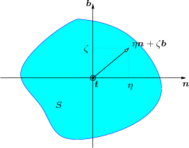
The geometric properties of the cross-section are determined by the following parameters (recall that the first moments of area,  and
and  , vanish, because the center of coordinates is the centroid of
  ):
):
- the area of
 :
: 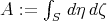 ;
; - the second moments of area with respect to the axis
 and
and  :
: 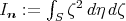 and
and 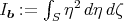 , respectively;
 - the polar moment of area:
 ;
;  .
.
These parameters are not necessarily constant, but they are assumed to vary smoothly along the rod. For a non-degenerate rod,  is bounded above and below far from zero. Consequently, the same happens for the area moments,
  ,
,  and
and  .
.
Remark 2.1. For any planar set  , there exists an orthogonal coordinate system, named the set of principal axes, such that
  vanishes when computed in these coordinates. For particularly symmetric geometries of
  , for instance when the cross-section of the rod is a circle or a square,
  vanishes in any orthogonal coordinate system. However, in general, there is no reason for
  and
and  to be principal axes, so that
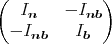
  does not necessarily vanish. In any case, it is straightforward to prove that the matrix
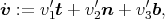
Vector fields defined on the line of centroids will be always written in the Frenet basis:

 ,
,  and
and  are not the components of
  in a fixed basis of
  , but in the Frenet basis
  , which changes from point to point of the curve.
 Since  ,
,  and
and  are smooth functions of the arc-length parameter
  , we have that

 | (2.1) |
then, by using the Frenet-Serret formulas (see, for instance, [2]), there holds
 |
where  and
and  are the curvature and the torsion of the rod, which are smooth functions of
  , too. Therefore,
  if and only if
  and
and  ,
,  .
.
Since we will confine our attention to elastic rods clamped at both ends, we proceed as in [2] and consider

![[∫ L ]1∕2 ∥v∥ := (|v|2 + |˙v|2) ds ; 1 0](/img/revistas/ruma/v49n1/1a0368x.png)
 is the space of vector fields defined on the line of centroids such that their components in the Frenet basis are in
  .
. We will systematically use in what follows the total derivative  . Since
  ,
,  and
and  are assumed to be smooth functions,
  is a norm on
  equivalent to
  (see [2, Theorem 3.1]). This is the reason why we denote
  the norm of
  . However, the total derivative
  should be distinguished from the vector
  of derivatives of the components of
  in the Frenet basis, as defined by (2.1).
The kinematic hypotheses of Timoshenko are used for the problem formulation. The deformation of the rod is described by the displacement of the line of centroids,  , and the rotation of the cross-sections,
  . The physical properties of the rod are determined by the elastic and the shear moduli
  and
and  , respectively, the shear correcting factors
  and
and  , and the volumetric density
  , all strictly positive coefficients. These coefficients are not necessarily constant; they are allowed to vary along the rod, but they are also assumed to be smooth functions of the arc-length
  .
.
We consider the problem of computing the free vibration modes of an elastic rod clamped at both ends. The variational formulation of this problem consists in finding non-trivial 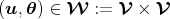 and
and  such that

where  is the vibration frequency and
  and
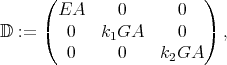
and  are the amplitudes of the displacements and the rotations, respectively (see [10]). The coefficients
  ,
,  and
and  are
are  matrices, which in the Frenet basis are written as follows:
 and the three matrices above are diagonal. We do not make this assumption in this paper.
 Remark 2.2. The vibration problem above can be formally obtained from the three-dimensional linear elasticity equations as follows: According to the Timoshenko hypotheses, the admissible displacements at each point  (see Fig. 2.1) are of the form
  , with
  ,
,  ,
,  and
and  being functions of the arc-length coordinate
  . Test and trial displacements of this form are taken in the variational formulation of the linear elasticity equations for the vibration problem of the three-dimensional rod. By integrating over the cross-sections and multiplying the shear terms by correcting factors
  and
and  , one arrives at problem (2.2).
It is well known that standard finite element methods applied to equations like (2.2) are subject to numerical locking: they lead to unacceptably poor results for very thin structures, unless the mesh-size is excessively small (see, for instance, [1]). This phenomenon is due to the different scales, with respect to the thickness of the rod, of the two terms on the left-hand side of this equation. An adequate framework for the mathematical analysis of locking is obtained by rescaling the equations in order to obtain a family of problems with a well-posed limit as the thickness becomes infinitely small.
With this purpose, we introduce the following non-dimensional parameter, characteristic of the thickness of the rod:
By defining

Problem (2.2) can be equivalently written as follows:
Problem  : Find non-trivial
  and
and  such that

The values of interest of  are obviously bounded above, so we restrict our attention to
 ![d ∈ (0, d ] max](/img/revistas/ruma/v49n1/1a03120x.png) . The coefficients of the matrices
. The coefficients of the matrices  ,
,  and
and  , as well as
  , are assumed to be functions of
  which do not vary with
  . This corresponds to considering a family of problems where the size of the cross-sections at all point of the line of centroids are uniformly scaled by
  , while their shapes as well as the geometry of the curve and the material properties remain fixed.
Remark 2.3. Matrices  ,
,  and
and  are positive definite for all
  , the last two because of Remark 2.1. Moreover, since all the coefficients are continuous functions of
  , the eigenvalues of each of these matrices are uniformly bounded below away from zero for all
  .
.
Remark 2.4. The eigenvalues  of Problem
  are strictly positive, because of the symmetry and the positiveness of the bilinear forms on its left and right-hand sides. The positiveness of the latter is a straightforward consequence of Remark 2.3, whereas that of the former follows from the ellipticity of this bilinear form in
  . This can be proved by using Remark 2.3 again and proceeding as in the proof of [2, Lemma 3.4 (a)], where the same result appears for particular constant coefficients (see also [6, Proposition 1]).
We introduce the scaled shear stress 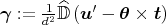 to rewrite Problem
  as follows:
![( ) [( ) ( ) ] ^𝔼 θ′,ψ ′ + (γ,v ′ - ψ × t) = λ ^Au, v + d2 ^𝕁θ, ψ ∀(v, ψ) ∈ W, γ = -1-^𝔻 (u′ - θ × t), d2](/img/revistas/ruma/v49n1/1a03139x.png)
where  denotes the
  inner product.
To analyze the approximation of this problem, we introduce the operator

defined by 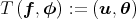 , where
  is the solution of the associated load problem:
The existence and uniqueness of the solution of this problem was analyzed in [2, Theorem 3.3] in case of particular constant coefficients and in [6, Proposition 2] for another equivalent formulation. Taking into account that (2.4) can be equivalently written as follows:

we note that the load problem falls in the framework of the mixed formulations considered in [5]. In this reference, the results from [1] are extended to cover this kind of problems. In particular, according to [5, Theorem II.1.2], to prove the well posedness it is enough to verify the classical properties of mixed problems:
- ellipticity in the kernel:
 such that

- inf-sup condition:
 such that
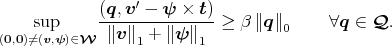
Property (i) has been proved in [2, Lemma 3.6] for  being the identity matrix. The extension to
  positive definite uniformly in
  is quite straightforward. Property (ii) has been proved in [2, Lemma 3.7]. An alternative simpler proof of an equivalent inf-sup condition appears in [6, Proposition 2].
Therefore, according to [5, Theorem II.1.2], problem (2.3)-(2.4) has a unique solution  and this solution satisfies
 |
Here and thereafter,  denotes a strictly positive constant, not necessarily the same at each occurrence, but always independent of
  and of the mesh-size
  , which will be introduced in the next section.
Because of the estimate above and the compact embedding  , the operator
  is compact. Moreover, by substituting (2.4) into (2.3), from the symmetry of the resulting bilinear forms, it is immediate to show that
  is self-adjoint with respect to the ‘weighted'
  inner product in the right-hand side of (2.3). Therefore, apart of
  , the spectrum of
  consists of a sequence of finite-multiplicity real eigenvalues converging to zero, all with ascent 1.
Note that  is a non-zero eigenvalue of Problem
  if and only if
  is a non-zero eigenvalue of
  , with the same multiplicity and corresponding eigenfunctions. Recall that these eigenvalues are strictly positive (cf. Remark 2.4).
Next, we define  by means of the limit problem of (2.3)-(2.4) as
  :
:

 is such that there exists
  satisfying:
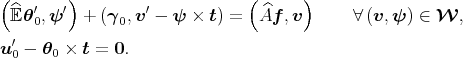
The above mentioned existence and uniqueness results from [2, Theorem 3.3] and [6, Proposition 2] covers this problem as well, in case of constant coefficients. As stated above, the proofs can be readily extended to our case.
It is proved in [9] that  converge in norm to
  . The next theorem follows from this fact and classical results from spectral perturbation theory (see [11]):
Lemma 2.1. Let  be an eigenvalue of
  of multiplicity
  . Let
. Let  be any disc in the complex plane centered at
  and containing no other element of the spectrum of
  . Then, for
  small enough,
  contains exactly
  eigenvalues of
  (repeated according to their respective multiplicities). Consequently, each eigenvalue
  of
of  is a limit of eigenvalues
  of
of  , as
, as  goes to zero.
Moreover, for any compact subset  of the complex plane not intersecting the spectrum of
  , there exists
  such that for all
  ,
,  does not intersect the spectrum of
  , either.
3. Finite elements discretization
Two different finite element discretizations of the load problem for Timoshenko curved rods have been analyzed in [2] and [6]. The two methods differ in the variables being discretized: the components of vector fields  in the Frenet basis,
  ,
,  and
and  , are discretized by piecewise polynomial continuous functions in [2]; instead, in [6], the discretized variable is the vector field
  . We follow the approach in [2].
Consider a family  of partitions of the interval
  ,
,  , with mesh-size
  . We define the following finite element subspaces of
  and
and  , respectively:
![V := {v ∈ V : v | ∈ P , j = 1,...,n, i = 1,2,3} , h { i[sj-1,sj] r } Qh := q ∈ Q : qi|[sj-1,sj] ∈ Pr-1, j = 1,...,n, i = 1,2,3 ,](/img/revistas/ruma/v49n1/1a03210x.png)
where  ,
,  , are the components of
  in the Frenet basis,
  are the spaces of polynomials of degree lower or equal to
  , and
, and  .
.
Let  . The following is the discrete vibration problem in mixed form:
Problem  : Find non-trivial
  and
and  such that:
![( ) [( ) ( ) ] ^𝔼 θ′,ψ ′ + (γ ,v ′- ψ × t) = λh A^uh, vh + d2 ^𝕁θh,ψ h h h h h h ∀ (vh,ψh ) ∈ Wh, ′ 2 ( -1 ) (uh - θh × t,qh) - d ^𝔻 γh,qh = 0 ∀qh ∈ Qh.](/img/revistas/ruma/v49n1/1a03221x.png)
In the same manner as in the continuous case, we introduce the operator

defined by  , where
 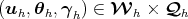 is the solution of the associated discrete load problem:
Problem (3.1)-(3.2) falls in the framework of the discrete mixed formulations considered in [5, Section II.2.4]. In order to apply Proposition II.2.11 from this reference to conclude well-posedness of this discrete problem and error estimates, it is enough to verify the following classical properties, for  small enough:
- ellipticity in the discrete kernel:
 , independent of
  , such that

- discrete inf-sup condition:
 , independent of
  , such that
Property (i) has been proved in [2, Lemma 4.2] for  being the identity matrix and
  sufficiently small. The extension to
  positive definite uniformly in
  is quite straightforward. Property (ii) has been proved in [2, Lemma 4.3]. An alternative simpler proof of this condition can be found in [9, Lemma 6.2].
On the other hand, (3.4) is obtained by adapting to our case the duality argument used to prove [6, Theorem 2]. Therefore, the following theorem follows:
Theorem 3.1. For sufficiently small  , problem (3.1)-(3.2) has a unique solution
 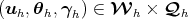 . This solution satisfies
 |
where  is independent of
  and
and  .
.
Let  be the solution of (2.3)-(2.4). If
  ,
,  , then

with  independent of
  and
and  .
.
By adding (3.1) and (3.2), from the symmetry of the resulting bilinear forms, it is immediate to show that  is self-adjoint with respect to the ‘weighted'
  inner product in the right-hand side of (3.1). Therefore, apart of
  , the spectrum of
  consists of a finite number of finite-multiplicity real eigenvalues with ascent 1.
Once more the spectrum of the operator  is related with the eigenvalues of the spectral problem
  :
:  is a non-zero eigenvalue of this problem if and only if
  is a non-zero eigenvalue of
  , with the same multiplicity and corresponding eigenfunctions. It is simple to prove that these eigenvalues are strictly positive. Moreover, the eigenvalues cannot vanish. In fact, according to the expression above, since
  and
and  are positive definite (see Remark 2.3),
  implies
  . Then, the second equation of Problem
  implies that
  and, hence,
  and
and  vanish because of property (i).
Our aim is to use the spectral theory for compact operators (see [3], for instance) to prove convergence of the eigenvalues and eigenfunctions of  towards those of
  . However, some further considerations will be needed to show that the error estimates do not deteriorate as
  becomes small. With this purpose, we will use the following result:
 |
which follows from (3.3) with  . As a consequence of this estimate,
  converges in norm to
  as
as  goes to zero. Hence, standard results of spectral approximation (see for instance [11]) show that if
  is an eigenvalue of
  with multiplicity
  , then exactly
  eigenvalues
  of
of  (repeated according to their respective multiplicities) converge to
  .
.
The estimate above can be improved when the source term is an eigenfunction  of
of  . Indeed, in such a case, for all
  and
and  sufficiently small,
 |
with  depending on
  and on the eigenvalue of
  associated with
  . Note that in principle the constant
  should depend also on
  , because the eigenvalue does it. However, according to Lemma 2.1, for
  sufficiently small we can choose
  independent of
  . Hence, from (3.3)-(3.4) with
  , we obtain:
We remind the definition of the gap or symmetric distance  between closed subspaces
  and
and  of
of  in norm
  ,
,  :
:

![[ ] ∥∥ ∥∥ δk(Y, Z ) := sup inf ∥(v - ^v,ψ - ^ψ )∥ . (v,ψ)∈Y (^v,^ψ)∈Z k ∥(v,ψ )∥k=1](/img/revistas/ruma/v49n1/1a03306x.png)
For the sake of simplicity we state our results for eigenvalues of  converging to a simple eigenvalue of
  as
as  . The following theorem yields
  -independent error estimates for the approximate eigenvalues and eigenfunctions. Its proof is a consequence of (3.5)-(3.6), [3, Theorem 7.1 and 7.2] and Lemma 2.1.
Theorem 3.2. Let  be an eigenvalue of
  converging to a simple eigenvalue
  of
of  as
as  tends to zero, Let
  be the eigenvalue of
  that converges to
  as
as  tends to zero. Let
  and
and  be the corresponding eigenspaces. Then, for
  and
and  small enough,
with  independent of
  and
and  .
.
This theorem yields optimal order error estimates for the approximate eigenfunctions in norms  and
and  . An optimal double order holds for the approximate eigenvalues. In fact, the following theorem has been proved in [9, Theorem 3.4] by adapting to our problem a standard argument for variationally posed eigenvalue problems (see [3, Lemma 9.1], for instance).
Theorem 3.3. Let  and
and  , with
  and
and  as in Theorem 3.2. Then, for
  and
and  small enough,
 independent of
  and
and  .
. We report in this section the results of a numerical test computed with a matlab code implementing the finite element method described above. We have used the lowest possible order:  ; namely, piecewise linear continuous elements for the displacements
  and the rotations
  , and piecewise constant discontinuous elements for the shear stresses
  .
.
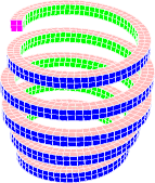
We have computed the vibration modes with lowest frequencies  for a helical rod. We have considered a helix with five turns, clamped at both ends. The equation of the helix centroids line parametrized by its arc-length is as follows:
 | (4.1) |
the curvature is  , the torsion
  , and the length of the eight-turns helix is
  . We have taken
  cm,
cm,  cm and a square of side-length
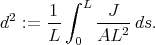
  cm as the cross section of the rod. Thus, the thickness parameter is in this case
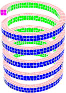
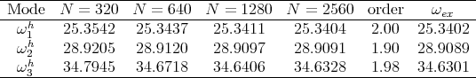
  . Figure 4.1 shows the undeformed helix.
|
We have computed the lowest vibration frequencies  by using uniform meshes of
  elements, with different values of
  . We have used the following physical parameters, which correspond to steel:
- elastic moduli:
 kgf/cm
 (
( );
); - Poisson coefficient:
 ;
; - density:
 kg/cm
kg/cm ;
; - correction factors:
 .
.
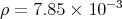
Since no analytical solution is available for this rod, we have estimated the order of convergence by means of a least squares fitting. Table 4.1 shows the lowest vibration frequencies computed on successively refined meshes. It also includes the computed orders of convergence and extrapolated ‘exact' vibration frequencies  .
.
|
To help identifying the different modes, we report three-dimensional plots of the deformed rods. With this purpose, we have used modulef to create an auxiliary hexahedral mesh of the actual three-dimensional rod and the displacements at each node of this auxiliary mesh have been computed from  and
and  as described in Remark 2.2. The resulting deformed rods have been plotted with modulef, too.
Figure 4.2 show the lowest-frequency vibration modes. The first one is a typical spring mode, the second one is an extensional mode, and the third one is a kind of ‘phone rope' vibration mode.
|
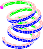
 (top),
  (middle) and
  (bottom).
[1] Arnold, D.N., Discretization by finite elements of a model parameter dependent problem. Numer. Math., 37 (1981) 405-421. [ Links ]
[2] Arunakirinathar, K., Reddy, B.D., Mixed finite element methods for elastic rods of arbitrary geometry, Numer. Math., 64 (1993) 13-43. [ Links ]
[3] Babuka. I., Osborn, J., Eigenvalue problems, in: Handbook of Numerical Analysis, Vol II. Ciarlet, P.G., Lions, J.L. (eds.), North Holland, Amsterdam, 1991, pp. 641-687. [ Links ]
[4] Babuka, I., Suri, M., On locking and robustness in the finite element method, SIAM J. Numer. Anal., 29 (1992) 1261-1293. [ Links ]
[5] Brezzi, F., Fortin, M., Mixed and Hybrid Finite Element Methods, Springer-Verlag, New York, 1991. [ Links ]
[6] Chapelle, D., A locking-free approximation of curved rods by straight beam elements, Numer. Math., 77 (1997) 299-322. [ Links ]
[7] Durán, R., Hervella-Nieto, L., Liberman, E., Rodríguez, R., Solomin, J., Approximation of the vibration modes of a plate by Reissner-Mindlin equations, Math. Comp., 68 (1999) 1447-1463. [ Links ]
[8] Durán, R., Hernández, E., Hervella-Nieto, L., Liberman, E., Rodríguez, R., Error estimates for low-order isoparametric quadrilateral finite elements for plates, SIAM J. Numer. Anal., 41 (2003) 1751-1772. [ Links ]
[9] Hernández, E., Otárola, E., Rodríguez, R., Sanhueza, F., Approximation of the vibration modes of a Timoshenko curved rod of arbitrary geometry, IMA J. Numer. Anal. (to appear). [ Links ]
[10] Karami, G., Farshad, M., Yazdchi, M., Free vibrations of spatial rods - a finite-element analysis. Comm. Appl. Numer. Methods, 6 (1990) 417-428. [ Links ]
[11] Kato, T., Perturbation Theory for Linear Operators, Springer Verlag, Berlin, 1995. [ Links ]
[12] Kikuchi, F., Accuracy of some finite element models for arch problems, Comput. Methods Appl. Mech. Engrg., 35 (1982) 315-345. [ Links ]
[13] Litewka, P., Rakowski, J., Free vibrations of shear-flexible and compressible arches by FEM., Internat. J. Numer. Methods Eng., 52 (2001) 273-286. [ Links ]
[14] Loula, A.F.D., Franca, L.P., Hughes, T.J.R., Miranda, I, Stability, convergence and accuracy of a new finite element method for the circular arch problem, Comput. Methods Appl. Mech. Engrg., 63 (1987) 281-303. [ Links ]
[15] Reddy, B.D., Volpi, M.B., Mixed finite element methods for the circular arch problem, Comput. Methods Appl. Mech. Engrg., 97 (1992) 125-145. [ Links ]
E. Hernández
Departamento de Matemática,
Universidad Técnica Federico Santa María,
Casilla 110-V, Valparaíso, Chile.
erwin.hernandez@mat.utfsm.cl
E. Otárola
Departamento de Matemática,
Universidad Técnica Federico Santa María,
Casilla 110-V, Valparaíso, Chile.
enrique.otarola@alumnos.utfsm.cl
R. Rodríguez
Departamento de Ingeniería Matemática,
Universidad de Concepción,
Casilla 160-C, Concepción, Chile.
rodolfo@ing-mat.udec.cl
F. Sanhueza
Departamento de Ingeniería Matemática,
Universidad de Concepción,
Casilla 160-C, Concepción, Chile.
rodolfo@ing-mat.udec.cl
Recibido: 10 de abril de 2008
Aceptado: 18 de abril de 2008

