Iterated Aluthge transforms: a brief survey

Jorge Antezana^*, Enrique R. Pujals^† and Demetrio Stojanoff^*

* Partially supported by CONICET (PIP 4463/96), Universidad de La Plata (UNLP 11 X472) and ANPCYT (PICT03-09521).
† Partially supported by CNPq

 Dedicated to the memory of Mischa Cotlar

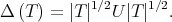
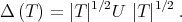
Abstract. Given an r × r complex matrix T, if is the polar decomposition of T, then the Aluthge transform is defined by

Let denote the n-times iterated Aluthge transform of T, i.e. and 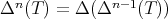, . In this paper we make a brief survey on the known properties and applications of the Aluthge trasnsorm, particularly the recent proof of the fact that the sequence converges for every r × r matrix T. This result was conjectured by Jung, Ko and Pearcy in 2003.

2000 Mathematics Subject Classification. Primary 37D10. Secondary 15A60.

Key words and phrases. Aluthge transform, stable manifold theorem, similarity orbit, polar decomposition.

1. Introduction

Let be a Hilbert space and a bounded operator defined on whose (left) polar decomposition is . The Aluthge transform of is the operator defined by

(1)

This transform was introduced in [1] by Aluthge, in order to study p-hyponormal and log-hyponormal operators. Roughly speaking, the idea behind the Aluthge transform is to convert an operator into another operator which shares with the first one some spectral properties but it is closer to being a normal operator.

The Aluthge transform has received much attention in recent years. One reason is its connection with the invariant subspace problem. Jung, Ko and Pearcy proved in [15] that has a nontrivial invariant subspace if an only if does. On the other hand, Dykema and Schultz proved in [10] that the Brown measure is preserved by the Aluthge transform. Another reason is related with the iterated Aluthge transform. Let and 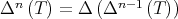for every . In [16] Jung, Ko and Peacy raised the following conjecture:

Conjecture 1. The sequence of iterates converges, for every matrix .     

This paper intends to give a brief survey on different properties of the Aluthge transform, making special emphasis on those results related with Conjecture 1, which was originally stated for operators on Hilbert spaces, and remains open for finite factors.

We begin the article with a historical summary that helps to explain the connection of the Aluthge transform with the invariant subspace problem and to describe some results that motivated and suggested that the conjecture might be true for operators on Hilbert spaces. Nevertheless, some couterexamples were found in this setting. We will expose one of them with some detail, which is particularly interesting because it shows an operator such that the sequence does not converge even in the weak operator topology.

In the second part of the article, we summarize two works ([6] and [8]) which contain a proof of a positive answer to Conjecture 1 and some results on the regularity of the limit function. In these papers a new approach, based on techniques from dynamical systems, is introduced. The most important result used is the so-called stable manifold theorem for pseudo-hyperbolic systems (briefly described in Appendix A). Using this dynamical approach Conjecture 1 is firstly proved in [6], for every diagonalizable matrix. In the second article [8], using again a dynamical approach, combined this time with geometrical arguments in order to manage some technical difficulties, Conjecture 1 is completely solved. Although we shall not describe it, we also refer to the reader to the work by Huajun Huang and Tin-Yau Tam [13], where some related results are shown using different techniques

We also include a section with some open problems regarding the continuity of the limit function and the convergence for some particular operators acting on infinite dimensional space. Finally, we add two appendices where we give the precise statements of the stable manifold theorem, and describe the geometrical properties of similarity and unitary orbits of matrices.

Notation. Throughout this paper denotes the algebra of complex matrices, the group of all invertible elements of , and the group of unitary operators. We denote is normal. If , we denote by the diagonal matrix with in its diagonal.

Given , denotes the spectrum of , the vector of eigenvalues of (counted with multiplicity), and the spectral radius of . We shall consider the space of matrices as a real Hilbert space with the inner product defined by . The norm induced by this inner product is the Frobenius norm, that is denoted by . For and , by means of we denote the distance between them, with respect to the Frobenius norm. If is a Hilbert space, denotes the algebra of bounded operators on .

2. Historical remarks

One of the most challenging problems in operator theory is the invariant subspace problem (ISP from now on). This problem states that every operator in has a non trivial invariant subspace. It is a property that has every operator in a (complex) finite dimensional space because of the existence of eigenvectors. It is not difficult to see that the ISP also has a positive answer if the underlying Hilbert space is not separable. However, for separable Hilbert spaces, the problem is still open.

Although the ISP is very difficult to deal with, it was proved that some particular classes of operators have many non-trivial invariant subspaces. One of the most important is the class of normal operators. Indeed, using the functional calculus developed by von Neumann, it can be proved that a normal operator has as many invariant subspaces. This suggested the idea of isolating some properties of normal operators that could be related with the fact of having invariant subspaces. This motivated the definition of hyponormal and p-hyponormal operators. Recall that, given a Hilbert space and , and operator is called -hyponormal (-hn) if

If , i.e., if for every , then is simply called hyponormal ().

In 1987, Brown was able to prove that every hyponormal operator whose spectrum has non-empty interior has a non trivial invariant subspace. In 1990, Aluthge considered the possibility of extending this result to p-hyponormal operator and defined what is now called Aluthge transform. The first result that caught the attention on this transformation is summarized in the following statement:

Theorem 2.1 (Aluthge [1]). Let be p-hyponormal. Then

• If , then is hn,
• If , then is -hn,
• It holds that is hn.    

Later on, Jung, Ko and Pearcy proved the next result that allowed to extend Brown's result to p-hyponormal operators:

Theorem 2.2 (Jung-Ko-Pearcy [15]). If denotes the lattice of invariant subspaces of a given operator , then .    

This result led to the first version of Jung-Ko-Pearcy conjecture on the iterated Aluthge transform sequence: The sequence of iterates converges to a normal operator for every . As soon as they raised this conjecture, many results supporting this conjecture appeared. The following formula for the spectral radius due to Yamazaki (see also Wang [19]) was one of the most important:

Theorem 2.3 (Yamazaki [21]). Given , then .    

However, after several positive partial results, some counterexamples appeared. One of the most interesting was found by Yanahida's [20]. Using a smart selection of weights, Yanahida defines a weighted shift operator whose sequence of iterated Aluthge transforms does not converge, even with respect to the weak operator topology! Let us briefly describe it: let be the canonical basis of , and the weighted shift operator defined by where

Straightforward computations show that is also a weighted shift with weights: , . Then, using some tricky estimates, it can be proved that the sequence does not converge, which implies that the sequence of iterates does not converge in the weak operator topology. After these counterexamples, the conjecture was restricted to matrices and takes the form stated in the introduction. Although the ISP has no sense for matrices, several authors have kept working on the conjecture in this setting because of the following reasons:

1. Despite the positive computational evidence, it was surprisingly difficult. For example, very complicated computations were needed to prove the case (see [3]).
2. It would be considered as a first step in order to get a characterization of the operators for which the sequence converges (see [14] and the references therein).
3. The conjecture remains open in the context of finite von Neumann factors (i.e. II factors), where the ISP has growing interest (see [10]).

We conclude this section with some results that have been very useful in order to study Conjecture 1. The first result is on the limit points of the iterated sequence. Note that, by Theorem 2.3, the sequence is bounded. Hence, if we restrict our attention to matrices, it has limit points. The following result, independently proved by Ando [2] and Jung, Ko and Pearcy [16], gives more details on them:

Proposition 2.4 (Ando, Jung-Ko-Pearcy). If , the limit points of the sequence are normal. Moreover, if is a limit point, then with the same algebraic multiplicity.    

Then, studying the Jordan structure of with respect with the Jordan structure of , the next reduction of the conjecture was proved in [5]:

Proposition 2.5. If the Aluthge transform sequence converges for every invertible matrix (resp. invertible diagonalizable matrix), then it does for every matrix (resp. diagonalizable matrix).    

These two results motivate us to consider the dynamical approach that will be described in the next section. In the next proposition we summarize some easy properties of the Aluthge transform which are necessary to understand this approach.

Proposition 2.6. Let . Then:

1. if and only if is normal.
2. for every .
3. for every .
4. . In [5] it is proved that equality holds only if .
5. and have the same spectrum and characteristic polynomial.
6. If then (orthogonal decompositions).    

We will also use systematically the following result on the regularity properties of on (see [10] or [6]):

Theorem 2.7. The map is continuous in and it is of class in .    

Remark 2.8. The map fails to be differentiable at several non invertible matrices.

 

3. Convergence results

Throughout this section, we fixe a matrix . We denote by , the vector of eigenvalues of (counted with multiplicity). In the following subsections (3.1 and 3.2) we shall describe briefly the proof of Conjecture 1, following the articles [6], for the diagonalizable case, and [8], for the general case. Let denote the set of diagonalizable matrices of .

3.1. The diagonalizable case. As we mentioned in the previous section, Conjecture 1 can be reduced to the invertible case. Since , it holds that So,

the similarity orbit of . This suggests that we can study the Aluthge transform restricted to , which has a rich geometric structure. In particular, it is a riemannian submanifold of (see Appendix B for more details).

If the Aluthge transform is studied restricted to the similarity orbit, the diagonalizable case has some advantages. Note that, if , then contains a compact submanifold of fixed points, and the sequence goes to this submanifold as . In fact, since , then for some diagonal matrix which has the same characteristic polynomial as . The unitary orbit of , is a compact submanifold of that consists of all normal matrices in . By Proposition 2.4, is fixed by the Aluthge transform and every limit points of the sequence belongs to . In contrast, if , then does not have fixed points, and the sequence of iterated Aluthge transforms still goes to , which is not contained in , but in its boundary. The key result in order to perform the dynamical approach to this problem is the following:

Theorem 3.1. Let be an invertible diagonal matrix. For every , there exists a subspace of the tangent space such that

1. ;
2. Both, and , are -invariant;
3. and , where

   

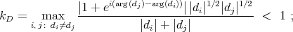
4. If satisfies , then .

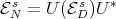In particular, the map 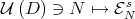is smooth. This fact can be formulated in terms of the projections onto parallel to , .    

The basic idea of the proof is that has an easy description in terms of coordinates (see Eq (4) in Appendix B). By a sequence of steps, one can describe , for , as a Hadamard multiplication , for a matrix . These facts allow to find the subspace as well as bounds for . The general case ( ) follows by unitary conjugations.

The idea behind Theorem 3.1 is the following: when we iterate the derivative of the Aluthge transform on an element of the tangent space of , for some , the sequence of iterates converge exponentially to . This is the behavior that one expects the Aluthge transform (instead of its derivative) to have. In order to extrapolate this result to the non-linear setting, we used the stable manifold theorem, which is a well known result of dynamical systems introduced independently by Hadamard and Perron (see Appendix). Under the conditions which Theorem 3.1 assures for the Aluthge transform, this theorem states that there exists a local submanifold through each such that:

1. , in particular is transversal to .
2. The submanifold is characterized as the set of matrices near that converge exponentially to by the iteration of the Aluthge transform.

Since the problem of the convergence of the iterates of the Aluthge transform has a symmetry due to the invariance by unitary conjugation, the size of the submanifolds as well as the exponential rate of convergence is uniform along the unitary orbit . These fact allow to prove, using arguments that involve the inverse mapping theorem, that the union of the submanifolds form an open neighborhood of (see Fig. 1). Thus, as the sequence goes toward , for some large enough the sequence of iterated Aluthge transforms enters into this open neighborhood, and, from that on, the sequence converges exponentially. Moreover, standard computations also show that the functional sequence converges uniformly on to a limit function, denoted by , which is a strong (continuous) retraction from onto .

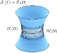
Figure 1: Union of stable manifolds

From the above mentioned facts, we can only deduce that is continuous. However, better regularity properties can be proved. Let be an open neighborhood of contained in the union of the submanifolds . As by the uniqueness of the limit, we can define a projection by:

It is not difficult to prove that this map is of class . Moreover, the limit function can be locally written as the composition of with . Since both functions are on , is also of class on .

Similar arguments, which involve a more specific version of the stable manifold theorem, allow to prove that the limit function is also when it is restricted to the open dense set consisting of those matrices have all their eigenvalues different.

3.2. The nondiagonalizable case. The non-diagonalizable case is different, since the geometry context of the problem is more complicated. Let be non diagonalizable and such that . Then is contained in the boundary of , which also contains the orbits of matrices with smaller Jordan forms than the Jordan form of . The boundary of can be thought as a sort of lattice of boundaries. Therefore, in order to prove Conjecture 1, the problem is set in a more appropriate context so that both cases, diagonalizable and non-diagonalizable can be analyzed together. In this new approach, the Aluthge transform is thought as an endomorphism of the open set , and all the orbits mentioned before are considered, not as a manifold, but as the basin of attraction of . By definition, in this case, the basin of attraction consists of those matrices such that the sequence goes to as . Note that, by Proposition 2.4, the basin can also be characterized as the set of those matrices that have the same characteristic polynomial as .

Since the Aluthge transform is thought as an endomorphism on the open set , the descomposition of Theorem 3.1 has to be extended to a decomposition of in -invariant subspaces, for each . This extension follows using that,

(2)

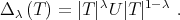
This fact can be proved by the standard properties of , since can be characterized as the commutant of . Hence, just take the decomposition . The stable manifold theorem used in this context is a standard extension to (see Remark A.4), and no differential structure is required in the basin. This theorem implies the existence of -invariant manifolds through each in the basin close enough to . One of the most important properties of these manifolds is that

(3)

where and are constants that only depend on the distance among different eigenvalues of . Hence, if the sequence converges for some , then the same must happen for (with the same limit).

In the diagonalizable case, we have considered only the stable manifolds for points and it was proved that the union of these manifolds contains an open neighborhood of in .

That approach fails in the general case, because the basin in not a manifold. So, a different idea is used. Inside the basin, there is a distinguished subset of matrices which satisfy Conjecture 1. This set, denoted by consists of those matrices, in the basin, with orthogonal spectral projections. Indeed, given , let be the spectrum of , the spectral projection of associated to each , and . Observe that is uniquely determined (as a normal matrix) by its vector and the spectral projections . But Proposition 2.4 assures that all the limit points of the sequence must be normal matrices with this vector, and item 6 of Proposition 2.6 assures that they must have the same spectral projections as (because they are orthogonal). Hence is the unique possible limit point, so that .

Having identified this set in the basin, the strategy is to prove that, for every in the basin near , the stable manifolds intersect the set . This fact would be enough by the remark which follows Eq. (3), and the previous study about .

However, does not have a differential structure, which is an important technical obstacle. To avoid this problem, the stable manifolds as well as are projected onto the orbit , using the above mentioned function , which is smooth (see Kato's book [17]). Observe that if and only if . On the other hand, the derivative of at is an orthogonal projection with range equal to . By a continuity argument, this implies that, for every close enough to , the nullspace of the derivative of at the different points of is transversal to the corresponding tangent spaces of . This implies that the projection onto of the manifolds are submanifolds of . Moreover, it can be proved that is "close" in some sense to , where is certain normal operator close to . Observe that is one of the stable manifolds studied in the diagonalizable case. Therefore intersects transversally . These facts imply, by some well known results about transversal intersections (see [11]), that also intersects . Finnaly, if , then is the projection of a matrix (see Fig. 2).

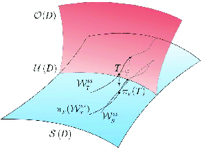
Figure 2: The projection argument

Similar (but slightly more complicated) arguments show that the limit map is continuous on . Nevertheless, the previous techniques are not useful to study continuity outside of because the map fails to be differentiable there.

Rate of convergence. In [6] it was proved that, if is diagonalizable, then after some iterations the rate of convergence of the sequence becomes exponential. More precisely, for some and every , there exist and such that . This exponential rate depends on the spectrum of . Actually, if for some diagonal matrix , then , the constant which appears in Theorem 3.1. Using the formula for , one can see that it is closer to (so that the rate of convergence becomes slower) if the different eigenvalues are closer one to each other.

These facts are no longer true if is not diagonalizable, since the rate of convergence for such a depends on the rate of convergence for some , which can be much slower (and not exponential). Observe that the proof of the convergence of the sequence , does not study the rate of convergence. It only shows that there exists an unique possible limit point for the sequence.

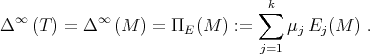
Nevertheless, if one denotes by the system of spectral projections of a matrix associated to its different eigenvalues, the previous approach shows that converges to exponentially, because . As in the case of diagonalizable matrices the rate of convergence of the spectral projections depends on the spectrum of , which agree with the spectrum of . Note that the spectrum of and the spectral projections of completely characterize the limit . Indeed, if , then

-Aluthge transform. Given and a matrix whose polar decomposition is , the -Aluthge transform of is defined by

All the results stated in this paper are also true for the -Aluthge transform for every , with almost the same proofs. Indeed, note that the basic results about Aluthge transform used throughout sections 3 and 4 are Theorem 3.1 and those stated in subsection 2.1. All these results were extended to every -Aluthge transform (see [5] and [7]). The unique difference is that the constant of Theorem 3.1 now depends on (see Theorem 3.2.1 of [7]). Anyway, the new constants are still lower than one for every . Moreover, they are uniformly lower than one on compact subsets of .

Another result which depends particularly on the Aluthge transform is Eq. (2), and the extended decomposition . Nevertheless, it is easy to see that both results are still true for every . On the other hand, the proof of the continuity of the map on uses the same facts about the Aluthge transform. So that, it also remains true for , for every . We resume all these remarks in the following statement:

Theorem 3.2. For every and , the sequence converges to a normal matrix . The map is continuous on .    

3.3. Some open problems. Concerning the convergence of iterated Aluthge sequences, the following problems are of great interest, and they still remain unsolved:

1. The continuity of the map . Using the techniques mentioned in this survey, it can be proved that this map is continuous in . But, as is not globally outside , new methods should be developed in order to prove the continuity of in . We remark that this fact is supported by computational evidence.
2. If is a separable Hilbert space, to get a characterization of those such that the sequence converges. The first step might be to study compact operators, using the convergence for matrices.
3. To prove that, if is a II factor (i.e. an infinite dimensional finite von Neumann algebra with trivial center), then the sequence converges to a normal element of , for every . This fact might be very important in order to get an affirmative answer of the ISP for these algebras, a problem which has great interest in operator theory and remains open. As in the case of compact operators, the finite dimensional case could be useful to prove Conjecture 1 in this setting, because there exist good finite dimensional methods of approximation for these particular class of von Neumann algebras.

 

Appendix A. The stable manifold theorem

As a general reference of this theory, we refer to the books [12] and [18]. Let be a smooth Riemann manifold and a submanifold (not necessarily compact). Throughout this subsection denotes the tangent bundle of restricted to .

Definition A.1. A pre-lamination indexed by is a continuous choice of a embedded disc through each . Continuity means that is covered by open sets in which is given by 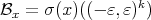where is a continuous section. Note that is a fiber bundle over whose projection is . Thus . If the sections mentioned above are , , we say that the pre-lamination is of class . A pre-lamination is called self coherent if the interiors of each pair of its discs meet in a relatively open subset of each one.

Theorem A.2 (Stable manifold theorem). Let be a endomorphism of and let be a compact subset of consisting of fixed points of . Assume that there exist two continuous subbundles of , denoted by and , such that, for every ,

1. .
2. is -invariant.
3. There exists such that .

Then, there is a continuous, -invariant and self coherent -pre-lamination (endowed with the -topology) such that, for every ,

1. ,
2. is tangent to ,
3. .    

Remark A.3. As is compact and , using the so-called -prelamination theorem, it can be proved that the prelamination is of class .

Remark A.4. Under the hypothesis of Theorem A.2, recall that the basin of attraction of is the set . Also recall that, for every , a local basin of is the set

Using standard arguments of dinamical systems, the distribution of subspaces and of Theorem A.2 can be extended to a local basin , for some small enough, so that the extended distribution of subspaces and satisfy:

1. .
2. is -invariant in the sense that .
3. There exists such that restricted to expand it by a factor greater than , and has norm lower than .

In this case, an extended version of the stable manifold theorem assures that there is a -pre-lamination which is continuous, -invariant, self coherent and satisfies for every (1) and (2) of Theorem A.2 and the following modified version of (3): .

 

Appendix B. Similarity orbit of a diagonal matrix

Let be diagonal, with , . By means of we denote the similarity orbit of , i.e., . On the other hand, denotes the unitary orbit of . We denote by the map defined by . With the same name we note its restriction to the unitary group: .

Proposition B.1 (See [9] or [4]). The similarity orbit is a submanifold of , and the projection becomes a submersion. Moreover, is a compact submanifold of , which consists of the normal elements of , and is a submersion.    

As a consequence of this result, it is not difficult to see that:

TD = {X ∈ : Xij = 0 for every (i,j) such that di = dj.}

(4)

Straightforward computations also show that, provided that . We consider on (and on ) the Riemannian structure inherited from (using the usual inner product on their tangent spaces). For , we denote by the Riemannian distance between and (in ). Observe that, for every , one has that and the map is isometric, on , with respect to the Riemannian metric as well as with respect to the metric of .

References

[1]    A. Aluthge, On p-hyponormal operators for , Integral Equations Operator Theory 13 (1990), 307-315.        [ Links ]

[2]    T. Ando, Aluthge Transforms and the Convex Hull of the Eigenvalues of a Matrix, Linear Multilinear Algebra 52 (2004), 281-292.        [ Links ]

[3]    T. Ando and T. Yamazaki, The iterated Aluthge transforms of a 2-by-2 matrix converge, Linear Algebra Appl. 375 (2003), 299-309.        [ Links ]

[4]    E. Andruchow and D. Stojanoff, Differentiable structure of similarity orbits, J. Operator Theory 21 (1989), 349-366.        [ Links ]

[5]    J. Antezana, P. Massey and D. Stojanoff, -Aluthge transforms and Schatten ideals, Linear Algebra Appl. 405 (2005), 177-199.        [ Links ]

[6]    J. Antezana, E. Pujals and D. Stojanoff, Convergence of iterated Aluthge transform sequence for diagonalizable matrices, Advances in Mathematics 216 (2007) 255-278.        [ Links ]

[7]    J. Antezana, E. Pujals and D. Stojanoff, Convergence of iterated Aluthge transform sequence for diagonalizable matrices II - -Aluthge transform, preprint available in arXiv.        [ Links ]

[8]    J. Antezana, E. Pujals and D. Stojanoff, The iterated Aluthge transforms of a matrix converge, preprint available in arXiv.        [ Links ]

[9]    G. Corach, H. Porta and L. Recht, The geometry of spaces of projections in C*-algebras, Adv. Math. 101 (1993), 59-77.        [ Links ]

[10]    K. Dykema and H. Schultz, On Aluthge Transforms: continuity properties and Brown measure, preprint available in arXiv.        [ Links ]

[11]    M. W. Hirsch, Differential topology, Graduate Texts in Mathematics 33, Springer-Verlag, New York 1994.        [ Links ]

[12]    M. W. Hirsch, C. C. Pugh, and M. Shub, Invariant manifolds, Lecture Notes in Mathematics, Vol. 583. Springer-Verlag, Berlin-New York, 1977.        [ Links ]

[13]    Huajun Huang and Tin-Yau Tam, On the Convergence of the Aluthge sequence, Oper. Matrices 1 (2007), no. 1, 121-141.        [ Links ]

[14]    M. Ito, T. Yamazaki and M. Yanagida, On the polar decomposition of the Aluthge transformation and related results, J. Operator Theory 51 (2004), no. 2, 303-319.        [ Links ]

[15]    I. Jung, E. Ko, and C. Pearcy, Aluthge transform of operators, Integral Equations Operator Theory 37 (2000), 437-448.        [ Links ]

[16]    I. Jung, E. Ko, and C. Pearcy, The Iterated Aluthge Transform of an operator, Integral Equations Operator Theory 45 (2003), 375-387.        [ Links ]

[17]    T. Kato, Perturbation theory for linear operators. Reprint of the 1980 edition. Classics in Mathematics. Springer-Verlag, Berlin, 1995.        [ Links ]

[18]    M. Shub, Global Stability of Dynamical Systems, Springer, 1986.        [ Links ]

[19]    D. Wang, Heinz and McIntosh inequalities, Aluthge Transformation and the spectral radius, Mathematical Inequalities and Applications Vol.6 No.1 (2003), 121-124.        [ Links ]

[20]    M. Yanagida , On convergence to n-th Aluthge transformation, unpublished, 2001.        [ Links ]

[21]    T. Yamazaki, An expression of the spectral radius via Aluthge tranformation, Proc. Amer. Math. Soc. 130 (2002), 1131-1137.        [ Links ]

Jorge Antezana
Departamento de Matemática,
Facultad de Ciencias Exactas,
Universidad Nacional de La Plata,
Calle 50 y 115, La Plata, Argentina
and IAM-CONICET
antezana@mate.unlp.edu.ar

Enrique R. Pujals
Instituto Nacional de Matemática Pura y Aplicada (IMPA),
Rio de Janeiro, Brasil
enrique@impa.br

Demetrio Stojanoff
Departamento de Matemática,
Facultad de Ciencias Exactas,
Universidad Nacional de La Plata,
Calle 50 y 115, La Plata, Argentina
and IAM-CONICET
demetrio@mate.unlp.edu.ar

Recibido: 10 de abril de 2008
Aceptado: 22 de abril de 2008