


Serviços Personalizados
Journal

Artigo
 Inglês (pdf)
 Artigo em XML
 Referências do artigo
 Enviar este artigo por email
Indicadores
-
 Citado por SciELO
Links relacionados
-
 Similares em
SciELO
Similares em
SciELO
Compartilhar

 Permalink
Revista de la Unión Matemática Argentina
versão impressa ISSN 0041-6932versão On-line ISSN 1669-9637
Rev. Unión Mat. Argent. v.49 n.1 Bahía Blanca jan./jun. 2008
Regular Optimal Control Problems with Quadratic Final Penalties
† Grupo de Sistemas No Lineales, INTEC (UNL-CONICET) Güemes 3450, 3000 Santa Fe, Argentina
‡ Centro de Matemática Aplicada, Escuela de Ciencia y Tecnología, UNSAM, M. de Irigoyen 3100, 1650 San Martín, Pcia. de Buenos Aires, Argentina
Hamilton's canonical equations (HCEs) have played a central role in Mechanics after (i) their equivalence with the principle of least action, and (ii) the variational calculus leading to the Euler-Lagrange equation, were established and applied (see [1]). Also, since the foundational work of Pontryagin [22], HCEs have been at the core of modern optimal control theory. When the problem concerning an  -dimensional control system and an additive cost objective is regular [19], i.e. when the Hamiltonian
  of the problem is smooth enough and can be uniquely optimized with respect to
  at a control value
  (depending on the remaining variables), then HCEs appear as a set of
  ordinary differential equations whose solutions are optimal state-costate time trajectories.
Concerning the infinite-horizon bilinear-quadratic regulator and change of set-point servo problems, there exists a recent attempt to find the missing initial condition for the costate variable, based on a state-dependent (generalized) algebraic Riccati equation (GARE) with solution  which allows to integrate the HCEs on-line with the underlying control process [9]. The same approach in a finite time-domain leads to a first-order partial differential equation (PDE) called ‘Generalized Differential Riccati Equation' (GDRE) (see [3], [6], [11]) for a time-state dependent matrix
  whose solution allows to calculate the missing initial costate
  and exhibits, for
  a limiting behavior (see [19]) similar to that of linear systems with the same cost, i.e.
 | (1) |
where  is the duration of each optimization process.
In the general nonlinear finite-horizon optimization set-up, allowing for a free final state, the cost penalty  imposed on the final deviation generates a two-point boundary-value situation. This is often a rather difficult numerical problem to solve. However, in the linear-quadratic regulator (LQR) case there exist well-known methods (see for instance [4], [24]) to transform the boundary-value into a final-value problem, related to the differential Riccati equation (DRE). Motivated by the role of Riccati equations, nonlinear situations have been treated for general final penalties by Byrnes [5], who posed a quasilinear first-order vector PDE (also labelled generalized Riccati equation by the author) for the optimal costate "in feedback form", i.e. as a function of the ‘event'
  but with boundary conditions on both
  and
and  . Its usefulness is still under discussion, since a discretization of the state-space is unavoidable for numerical treatment. The same question in the one-dimensional case and for a quadratic
  (in this paper it will always be
  has been extended to a whole
  -family of problems (see [7], [12]), generating two first-order, quasilinear, uncoupled PDEs with classical initial conditions, where the dependent variables are the missing boundary conditions
  and
and  of the HCEs. This approach has been completely disjoint from Riccati equations, but more in the line of the early invariant-imbedding ideas introduced by Bellman [2], [23]. Analogous ideas were retaken and reformulated for the multidimensional case, in the light of symplectic properties inherent to Hamiltonian dynamics. The resulting matrix and vector PDEs are under review [8] and will be just summarized here, together with still unpublished feedback expressions for the optimal control.
When the  -minimal control
  is not explicitly known, then new but similar PDEs appear, involving also the final value
  of the optimal control. The discussion of these equations would exceed the scope of this paper (see however [13], [14]).
After the relevant mathematical objects associated with the finite-horizon control problem are presented in Section 2, then the immersion into a family of  -processes is worked out in Section 3. Afterwards, in Section 4 the main PDEs for the missing boundary conditions are substantiated. A brief discussion on the potentiality for feedback control follows in Section 5, applications are then developed in Section 6, and finally the conclusions and perspectives are summarized.
In what follows only initialized, autonomous (for simplicity) control systems of the form
 | (2) |
will be considered. The state  moves into some region
  of
of  and the admissible control strategies are the real, piecewise continuous functions of the time-domain
  into some open subset
  of
of  . The right-hand side
  is assumed to be smooth enough as to guarantee existence and uniqueness of solutions to the dynamics' equation (2) in the range of interest. The (finite-horizon) quadratic final penalty optimization context will imply here that a cost functional like
 | (3) |
has to be minimized on the set of admissible control trajectories, where 
![= [0,T ],T < ∞,](/img/revistas/ruma/v49n1/1a0537x.png)
 is a nonnegative smooth function called ‘the Lagrangian' of the problem, and
  is a nonnegative-definite symmetric matrix called ‘the final penalty coefficient'. The ‘value function'
  can always be defined for such a problem, namely
![V (t,x ) ≜ inuf(⋅)J (T,t,x,u(⋅)),t ∈ [0,T ]](/img/revistas/ruma/v49n1/1a0541x.png) | (4) |
and, if the problem has a unique solution, then this solution is called ‘the optimal control strategy' 
 | (5) |
which in turn will generate ‘the optimal state trajectory'
 | (6) |
The Hamiltonian of such a problem is defined as usual,
 | (7) |
where  is called the ‘costate',
 ranging in
  -dimensional ‘phase-space'. Since
  is assumed regular, then there exists a unique
  -optimal control
 | (8) |
‘Explicitly regular' Hamiltonian means that the function  is known (not only its existence but also its explicit form) and that it is sufficiently smooth on its variables. The control Hamiltonian,
 | (9) |
gives rise to the HCEs (see [22] for general problems; [24], page 406 for the free final state case)
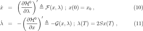
that is a  -dimensional ODE for a (Hamiltonian) vector field
  ,
,
 | (12) |
Solutions to Eqns. (10, 11) result, under the hypotheses made, the optimal state and costate trajectories (denoted  and
and  respectively), which are also related through the value-function by
 | (13) |
It is useful to remind also that the control Hamiltonian is constant along the optimal trajectories, since
![( 0) ′ ( 0) ′ d-H0 (x*(t),λ *(t)) = ∂H--- ⋅ F + ∂H--- ⋅ [- G ] = 0 . dt ∂x ∂ λ](/img/revistas/ruma/v49n1/1a0562x.png) | (14) |
3. Imbedding the problem into a  -family
The following notation for the missing boundary conditions will be used in this Section
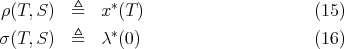
(the notation 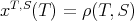 and
and 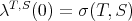 may eventually emphasize that the quantities refer to a particular
  -problem)
By assuming that the Hamiltonian vector field is at least  , then the existence of a flow
 | (17) |
is guaranteed, where  are appropriate regions of
  The flow verifies

where  is preferred to the usual
  to avoid confusions.
By calling  to the
  -advance transformations associated with the flow, the following identities become clear
 | (20) |
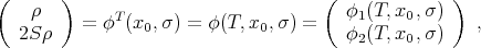
where  denote the ‘components' of the flow over the state and costate subspaces, respectively. The first component of Eq. (18) reads
 | (21) |
and similarly for the second component, in brief
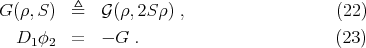
The (phase-space) derivative of the  -advance function will be needed in the sequel, so a special name is given to it and to its partitions
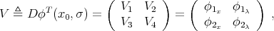 | (24) |
where  and so on. Existence and uniqueness of solutions imply that the inverse of
  exists and verifies
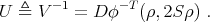 | (25) |
4. The main PDEs for missing boundary conditions
Hamiltonian vector fields have flows with the following important properties (see [18], page 378; [20], page 220)
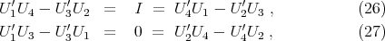
where the following notation is adopted for submatrices: 
Since the same is true for  its inverse can be calculated in terms of the submatrices
  namely
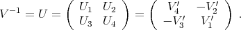 | (28) |
Now by deriving the first component of Eq. (20) with respect to 
 | (29) |
which will be written (with 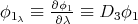 ) simply as
 | (30) |
and similarly, for the second component,
 | (31) |
The following operations over Eqns. (30, 31) use the symplectic properties of the vector field
 | (32) |
By repeating the procedure for the  -derivatives, analogous equations are obtained, namely
and from their combination,
 | (35) |
Now, by using  and properties in Eqns. (26, 27), together with results in Eqns. (32, 35), then a condensed form for previous identities is obtained
 | (36) |
which means that there really are only two independent first-order vector PDEs for  namely
Notice that only  and
and  are involved, although a pair of equivalent PDEs can be obtained involving
  and
and  In the one-dimensional case these equations can be uncoupled, obtaining (see [7])
but for  a more involved treatment is needed, as will be shown below.
For an  -dimensional state space it will be convenient to assign a name to the combined variable
  Eq. (18) can be written
 | (41) |
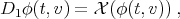
and by taking derivatives on both members with respect to  i.e.
i.e.  and then interchanging the order of derivation, the ‘variational equation' (see for instance [16], page 299) is obtained, namely
![D [D φ(t,v)] = DX (φ(t,v)) ⋅ D φ (t,v ) , 1 2 2](/img/revistas/ruma/v49n1/1a05115x.png) | (42) |
or, by abusing notation ( the symbol
  is reserved for
  )
)
 | (43) |
with the initial condition
 | (44) |
Actually, this means that  the fundamental solution of (43), which verifies (see [24], page 488)
 | (45) |
i.e. the following identity is established
 | (46) |
or, in short, reserving the symbol  for
for 
 | (47) |
Now, inspired in the treatment of the LQR in Hamiltonian form (see [4], [24]), two auxiliary matrices will be defined
 | (48) |
and deriving them with respect to  and using Eqns. (28, 47, 48),
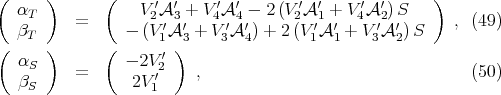
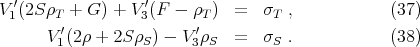
then the following identities are obtained
 | (51) |
 | (52) |
where the new matrices  take the form
Since for a process of zero duration,  then in such case
 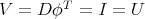 , and therefore the main matrix PDEs in Eq. (52) are subject to the initial conditions
 | (55) |
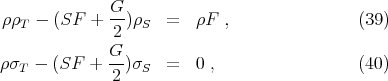
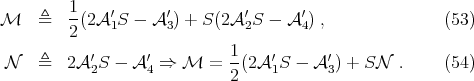
Now, Eqns. (53, 54) still include the unknown final state  inside the
  s so the (matrix) PDEs in Eq. (52) can not be solved alone. But, having found expressions for the partitions of
  in terms of the auxiliary matrices
  and their derivatives, (vector) Eqns. (37, 38) turn into
 | (56) |
which become solvable, at least in principle, when coupled to the matrix PDEs for  and subject to initial conditions
 | (57) (58) |
In short, the problem requires to solve in parallel two matrix first-order PDEs for  and another two vector first-order PDEs for
  , all meeting appropriate initial conditions. If instead of
  the remaining submatrices
  were chosen, then Eqns. (32, 35) take also a condensed form, namely
 | (59) |
but  can not be directly recuperated from them.
Concerning the existence and uniqueness of solutions to the coupled system of Eqns. (52, 56), there exist only local results (see [15], page 51), although the field of vector and matrix PDEs integration is in active development (see for instance [25]).
Let us denote as  the optimal initial costate corresponding to a
  -problem with initial state
  Smooth dependence on initial conditions for ODEs [16], extensive to first-order quasilinear PDEs [15], guarantees smooth dependence of
  on
on  Neither the matrix nor the vector PDEs developed in the previous section depend explicitly on
  The initial state
  only affects solutions through the conditions (57, 58). As a consequence, numerical software can sometimes handle this dependence "analytically", i.e. considering
  as a dummy variable when solving for
  So it will be assumed that
  is available for some appropriate open set
  containing the "expected perturbations" from the optimal state trajectory
 ![{x*(t),t ∈ [0,T]}](/img/revistas/ruma/v49n1/1a05161x.png) starting at the original fixed initial condition
starting at the original fixed initial condition 
 Under these assumptions it is clear that the optimal costate trajectory must also verify (analogously to the Dynamic Programming Principle for the value function)
![λ*(t) = σ(T - t,S, x*(t)) ∀t ∈ [0,T] .](/img/revistas/ruma/v49n1/1a05164x.png) | (60) |
Therefore, if at some intermediate time  the measured (or observed) state is
  possibly different from the expected but still inside
  a new optimal control problem starting at
  as initial condition (and duration
  may be considered to cope with state perturbations, and it follows that the new optimal control can be expressed in feedback form as
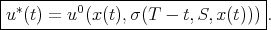 | (61) |
6.1. The (constant coefficient) LQR problem revisited. The Hamiltonian form of the LQR problem (with linear dynamics  and quadratic Lagrangian
  ) reads
 | (62) |
where 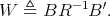 Therefore in this case the HCEs become a linear, time-constant dynamical system or vector field
  , whose flow verifies
 | (63) |
and consequently
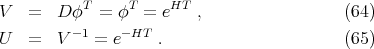
The following identities are easily obtained
Therefore, Eqns. (52) for  can be integrated alone, since they do not depend on
  Actually, from
 | (69) |
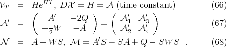
it follows that no further equations are needed for  Since
Since  is always invertible (see [24], p.371), then the missing boundary conditions result

Illustrations can be found in [10]. From Eq. (13) for the LQR case, the initial costate has here the form
 | (72) |
where  is in turn the numerical solution of the DRE, i.e. the final-value matrix ODE
 | (73) |
Therefore, from Eq. (71), for each  -problem the Riccati matrix
  should also verify
![1 -1 P(0) = -β(T, S)[α(T, S)] . 2](/img/revistas/ruma/v49n1/1a05190x.png) | (74) |
The method based on PDEs for missing boundary conditions avoid solving DRE for each particular  -problem, and storing, necessarily as an approximation, the Riccati matrix
  for the values of
 ![t ∈ [0,T ]](/img/revistas/ruma/v49n1/1a05193x.png) chosen by the numerical integrator, possibly different from the time instants for which the control
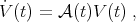
chosen by the numerical integrator, possibly different from the time instants for which the control  is constructed. Instead, the HCEs (62) can be integrated with initial conditions
 | (75) |
and the optimal trajectories  obtained for
  which allows to generate the optimal control at each time
 | (76) |
or, in this case, the feedback form, which becomes directly available due to the linear dependence of Eqns. (70, 71) on initial conditions,
![u *(t) = - 1R -1B ′β(T - t,S )[α (T - t,S)]-1 x . 2](/img/revistas/ruma/v49n1/1a05199x.png) | (77) |
As a side-product, an alternative formula for the Riccati matrix results:
![1 - 1 P (t) = -β(T - t,S)[α(T - t,S )] ∀t ∈ [0,T ]. 2](/img/revistas/ruma/v49n1/1a05200x.png) | (78) |
6.2. Bilinear systems and quadratic costs. The bilinear-quadratic case (with  will be used to illustrate the application of previous results to nonlinear systems. The dynamics and trajectory cost will be, respectively,
 | (79) |
The  -optimal control is readily obtained (see [24])
 | (80) |
and then the control Hamiltonian takes the form
![0 ′ ′ 1 ′ 2 H (x, λ) = x Qx + λ Ax - ---[λ (b + N x)] . 4r](/img/revistas/ruma/v49n1/1a05205x.png) | (81) |
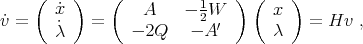
The HCEs are therefore
 = Ax - 2W (x )λ ,](/img/revistas/ruma/v49n1/1a05206x.png) | (82) |
![′ λ′(b + N x) ′ [ ]′ ˙λ = - 2Qx - A λ + ----------N λ = - 2Qx - A¯(x, λ) λ , 2r](/img/revistas/ruma/v49n1/1a05207x.png) | (83) |
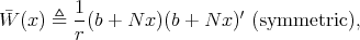
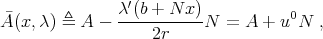
where the  -dependent matrix
  is clearly a generalization of the
  defined for linear systems, and analogously for
 | (84) |
 | (85) |
allowing to write the vector field  and its derivative
  in concise expressions, namely
![( ) ( ) A - 1W¯ (x ) x X (x,λ) = - 2Q - [2 ¯A(x,λ )]′ λ ,](/img/revistas/ruma/v49n1/1a05216x.png) | (86) |
![( ˆ 1 ¯ ) A (x,λ) -[ 2W (x)] ′ DX (x, λ) = - 2 ˜Q(λ ) - ˆA((x,λ ) ,](/img/revistas/ruma/v49n1/1a05217x.png) | (87) |
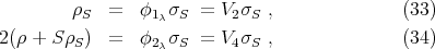
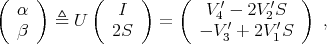
where new generalizations of LQR matrices appear,

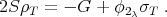
The matrix  can be evaluated by looking to the final conditions, i.e.
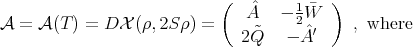 | (90) |
![W¯ = 1(b + N ρ)(b + N ρ)′ , (91 ) r ˆ 1- ′ ′ A = A - r[ρ S(b + N ρ)N + (b + N ρ)ρ SN ] , (92 ) 1 Q˜ = Q + --N ′S ρρ′SN . (93 ) r](/img/revistas/ruma/v49n1/1a05221x.png)
In conclusion, the relevant objects read in this case
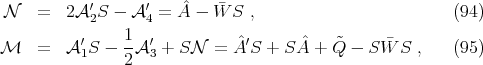
![[ ] 1- ′ F = A - r(b + N ρ)(b + N ρ) S ρ , (96 ) [ ′ ] G = 2 Q + A ′S - ρS-(b +-N-ρ)N ′S ρ . (97 ) r](/img/revistas/ruma/v49n1/1a05223x.png)
The following checking procedure can be performed over numerical solutions. It is known (see [6]) that the value function verifies, for the finite-horizon bilinear-quadratic problem,
![∂VT,S-(t,x) = 2[PT,S(t,x)]x , ∂x](/img/revistas/ruma/v49n1/1a05224x.png) | (98) |
for some matrix  solution of a generalized Riccati differential equation (GDRE), actually a first-order PDE in the variables
  that in the one-dimensional case takes the form
![[ ] [pt + F(x,p ) ⋅ px]x + pF (x,p) + 1G (x,p) = 0 , 2](/img/revistas/ruma/v49n1/1a05227x.png) | (99) |
with  as defined in Eqns. (21, 22), respectively.
It is also known (see [9], and [19] for the linear analogue) that for  the solutions to GDRE are compatible with solutions
  to the generalized algebraic Riccati equation (GARE) arising in the infinite-horizon case, namely
 | (100) |
via the limiting behavior
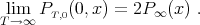 | (101) |
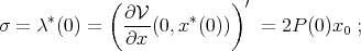
Numerical calculations performed for increasing time-spans (approximately) confirm the asymptotic result
![∂V σ ∞ = lim σ(T,0) = lim ---T,0(0,x0) = T→ ∞ [ T →∞] ∂x = lim 2 PT,0(0,x0) x0 = 2 [P ∞ (x0)]x0 . (102 ) T→ ∞](/img/revistas/ruma/v49n1/1a05233x.png)
7. Conclusions and perspectives
The solutions to the PDEs established in the previous Sections allow to transform the classical boundary-value problem posed for Hamilton equations in  dimensions, into an initial-value situation when the Hamiltonian is regular. This allows in turn to numerically integrate the original HCEs on-line with the control process, and to continuously construct the manipulated variable
 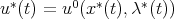 from the state and costate values provided by this integration, since the
  -optimal control function
  is known. The on-line accessibility to an accurate value for the optimal state is most valuable in practical situations, since physical states of nonlinear control systems are hardly available at all desired times. Sometimes even a feedback control form can be constructed from the solutions to the quasilinear PDEs.
The PDEs' method solves a whole family of  problems, avoiding additional off-line calculations and burdensome storing of information for each particular situation, as in methods of the DRE or GDRE type. The numerical integration of the new PDEs is relatively simple when only scalar values for
  are admitted, which is enough in many practical situations. Also, solutions providing the missing boundary conditions can be checked in several ways, and eventually iterated until convergence before using them to start controlling in real time.
Having the values of  for a wide range of
  parameter values may be helpful at the design stage. From one side, the values of
  can be reconsidered by the designer when acknowledging the final values of the state
  that will be obtained under present conditions. And if a change in the parameter values is decided, then it will not be necessary to perform additional calculations to manage the new situation. Besides, the value of
  is an accurate measure of the ‘marginal cost' of the process, i.e. it measures how much the optimal cost would change under perturbations, which can also influence the decision on adopting the final
  values.
Other than the possibility of integrating HCEs on-line with the real plant (and constructing the optimal control for the model in real time), or even the possibility of generating a feedback law as we shall see, the approach presented in this paper may also be useful when studying input-output  -stability of control systems, since the trajectory cost
![∫T [ 2 2 2] ∥y(t)∥ - γ ∥u(t)∥ dt 0](/img/revistas/ruma/v49n1/1a05247x.png) | (103) |
may be analyzed in this set-up for variable gain  even for nonlinear observation functions
 | (104) |
and nonlinear dynamics (see [17], [21]), provided the resulting Hamiltonian is regular. Therefore, these PDEs seem to provide a novel environment where to explore the balance ‘performance versus stability'.
Other aspects of this approach deserve research. For instance, the curves  are potentially a safeguard against Hamiltonian systems' instabilities (their linearizations have eigenvalues with positive real parts, because those associated with
  are symmetric to those corresponding to
  ). Therefore, it will probably add to robustness to construct the control by imposing a bound on costates
  for instance impeding the costates to trespass the reverse
  curve starting from
  when a finite horizon of duration
  is being optimized.
[1] Arnold, V.I., Mathematical Methods of Classical Mechanics, Springer-Verlag, New York, 1978. [ Links ]
[2] Bellman, R., Kalaba, R., A Note on Hamilton's Equations and Invariant Imbedding. Quarterly of Applied Mathematics, XXI:166-168, 1963. [ Links ]
[3] Bergallo, M., Costanza, V., Neuman, C.E., La Ecuación Generalizada de Riccati en Derivadas Parciales. Aplicación al Control de Reacciones Electroquímicas. Mecánica Computacional, XXV:1565-1580; 2006. [ Links ]
[4] Bernhard P., Introducción a la Teoría de Control Óptimo, Cuaderno del Instituto de Matemática "Beppo Levi" No 4, Rosario, Argentina, 1972. [ Links ]
[5] Byrnes, C., On the Riccati Partial Differential Equation for Nonlinear Bolza and Lagrange Problems, Journal of Mathematical Systems, Estimation, and Control 8(1)1-54, 1998. [ Links ]
[6] Costanza, V., Optimal State-Feedback Regulation of the Hydrogen Evolution Reactions, Latin American Applied Research, 35(4)327-335, 2005. [ Links ]
[7] Costanza, V., Finding initial costates in finite-horizon nonlinear-quadratic optimal control problems, Optimal Control Applications & Methods, 29(3)225-242; 2008. [ Links ]
[8] Costanza, V., Spies, R.D., Missing Boundary Conditions for Hamilton Canonical Equations in Optimal Control Problems, submitted to SIAM Journal on Control and Optimization, 2008. [ Links ]
[9] Costanza, V., Neuman C.E., Optimal Control of Nonlinear Chemical Reactors via an Initial-Value Hamiltonian Problem, Optimal Control Applications & Methods, 27:41-60, 2006. [ Links ]
[10] Costanza, V., Neuman C.E., Partial Differential Equations for Missing Boundary Conditions in the Linear-Quadratic Optimal Control Problem, Proc. XII Reunión RPIC, published in CD format, Río Gallegos, Argentina, 2007; selected for eventual publication in Latin American Applied Research, presently under review. [ Links ]
[11] Costanza, V., Picó, M., Control Hamiltoniano de Sistemas No Lineales en Tiempo Real; Proc. XI Reunión RPIC, published in CD format, Río Cuarto, Argentina, 2005. [ Links ]
[12] Costanza, V., Rivadeneira, P.S., Finite-Horizon Dynamic Optimization of Nonlinear Systems in Real Time. To be published in Automatica, 2008, DOI information: 10.1016/j.automatica.2008.01.033. [ Links ]
[13] Costanza, V., Rivadeneira, P.S., Regular Hamiltonian Problems with Implicit H-Optimal Control, Proc. XII Reunión RPIC, published in CD format, Río Gallegos, Argentina, 2007. [ Links ]
[14] Costanza, V., Rivadeneira, P.S., Minimal-Power Control of Electrochemical Hydrogen Reactions, submitted to Optimal Control Applications & Methods, 2008; under review. [ Links ]
[15] Folland, G.B., Introduction to Partial Differential Equations, 2nd. edition, Princeton University Press, Princeton, U.S.A., 1995. [ Links ]
[16] Hirsch, M.W. and S. Smale, Differential Equations, Dynamical Systems, and Linear Algebra, Academic Press, New York, 1974. [ Links ]
[17] Isidori, A., Nonlinear Control Systems II, Springer-Verlag, London, 1999. [ Links ]
[18] Jacobson, N., Basic Algebra I, W.H. Freeman and Company, San Francisco, U.S.A., 1974. [ Links ]
[19] Kalman, R.E., Falb, P.L., Arbib, M.A., Topics in Mathematical System Theory. McGraw-Hill, New York, 1969. [ Links ]
[20] Katok, A. and B. Hasselblatt, Introduction to the Modern Theory of Dynamical Systems, Cambridge University Press, Cambridge, U.K., 1999. [ Links ]
[21] Khalil, H.K., Nonlinear Systems. Prentice-Hall, 3rd Edition, Upper Saddle River, New Jersey, U.S.A., 2002. [ Links ]
[22] Pontryagin, L.S., Boltyanskii, V.G., Gamkrelidze, R.V., Mischenko, E.F., The Mathematical Theory of Optimal Processes. Wiley, New York, 1962. [ Links ]
[23] Sage, A.P., White, C.C, Optimum Systems Control. Prentice-Hall, 2nd Edition, Englewood Cliffs, U.S.A., 1977. [ Links ]
[24] Sontag, E.D., Mathematical Control Theory, Springer, 2nd Edition, New York, 1998. [ Links ]
[25] Zenchuk, A.I. and P.M. Santini, Dressing method based on homogeneous Fredholm equation: quasilinear PDEs in multidimensions, http://arxiv.org/pdf/nlin/0701031, 2007. [ Links ]
Vicente Costanza
INTEC, UNL-CONICET,
Güemes 3450,
3000 Santa Fe, Argentina
tsinoli@ceride.gov.ar
Recibido: 10 de abril de 2008
Aceptado: 18 de abril de 2008

