


Servicios Personalizados
Revista

Articulo
 Inglés (pdf)
 Articulo en XML
 Referencias del artículo
 Enviar articulo por email
Indicadores
-
 Citado por SciELO
Links relacionados
-
 Similares en
SciELO
Similares en
SciELO
Compartir

 Permalink
Revista de la Unión Matemática Argentina
versión impresa ISSN 0041-6932versión On-line ISSN 1669-9637
Rev. Unión Mat. Argent. v.49 n.2 Bahía Blanca jul./dic. 2008
A Model for the Thermoelastic Behavior of a Joint-Leg-Beam System for Space Applications
E.M. Cliff, Z. Liu and R. D. Spies*
Abstract. Rigidizable-Inflatable (RI) materials offer the possibility of deployable large space structures (C.H.M. Jenkins (ed.), Gossamer Spacecraft: Membrane and Inflatable Structures Technology for Space Applications, Pro-gress in Aeronautics and Astronautics, 191, AIAA Pubs., 2001) and so are of interest in applications where large optical or RF apertures are needed. In particular, in recent years there has been renewed interest in inflatable-rigidizable truss-structures because of the efficiency they offer in packaging during boost-to-orbit. However, much research is still needed to better understand dynamic response characteristics, including inherent damping, of truss structures fabricated with these advanced material systems. One of the most important characteristics of such space systems is their response to changing thermal loads, as they move in and out of the Earth's shadow. We study a model for the thermoelastic behavior of a basic truss componentconsisting of two RI beams connected through a joint subject to solar heating. Axial and transverse motions as well as thermal response of the beams with thermoelastic damping are taking into account. The model results in a couple PDE-ODE system. Well-posedness and stability results are shown and analyzed.
Key words and phrases. Truss structures, Euler-Bernoulli beams, thermoelastic system.
* Corresponding author
In recent years there has been renewed interest in Rigidizable-Inflatable (RI) space structures because of the efficiency they offer in packaging during boost-to-orbit. RI materials offer the possibility of deploying large space structures ([7]) and so are of interest in applications where large optical or RF apertures are needed. Several proposed space antenna systems will require ultra-light trusses to provide the "backbone" of the structure (see Figure 1(a)). It has been widely recognized that practical precision requirements can only be achieved through the development of new high-fidelity mathematical models and corresponding numerical tools.
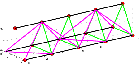 (a) Rigidizable-Inflatable truss structure (a) Rigidizable-Inflatable truss structure |
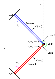 (b) Basic structure of the joint-legs-beams system (b) Basic structure of the joint-legs-beams system |
| Figure 1.1: Truss (a) and basic structure of the joint-legs-beams system (b). |
In this paper we study the dynamics of a basic truss component consisting of two RI beams connected through a joint (see Figure 1(b)). One of the more important characteristics of such space systems is their response to changing thermal loads, as they move in and out of the Earth's shadow. In this paper we study the thermoelastic behavior of a two-beam truss element subject to solar heating. The beams are fabricated as thin-walled circular cylinders.
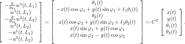
The equations of motion for the Joint-Leg-Beam system depicted in Figure 1(b) are the following (see [1] for details):
 (2.1) (2.1) |
![2 M d-[ x(t)y(t)θ1(t)θ2(t) ]T = C [ M1 (t)N1 (t)M2 (t)N2 (t)F1(t)F2 (t) ]T dt](/img/revistas/ruma/v49n2/2a075x.png) (2.2) (2.2) |
for time  and spatial variable
 ![si ∈ [0,Li]](/img/revistas/ruma/v49n2/2a077x.png) , where
, where  and
and  are
are  and
and  matrices give by
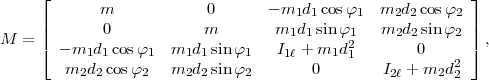 (2.3) (2.3) |
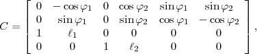 (2.4) (2.4) |
and the other functions and parameters are as follows (here the supra or sub-index  ,
,  will always refer to beam or leg
  ):
):  longitudinal and transversal displacement of the beam;
  horizontal and vertical displacement of the joint's tip;
  rotation angle of the leg;
  mass density, cross section area, length, Young's modulus, moment of inertia of the beam;
  mass, center of mass, length, moment of inertia of the leg;
  mass of the joint,
  ;
;  initial angle of leg
  with positive
  axis;
axis;  initial angle of leg
  with negative
  axis;
axis;  extensional force of beam at the end
  ;
;  shear force of beam at the end
  ;
;  bending moment of beam at the end
  .
.
Each beam is clamped at the end  . Thus the boundary conditions at
  are
are
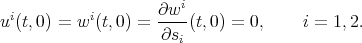 (2.5) (2.5) |
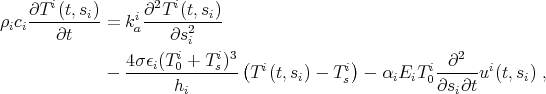
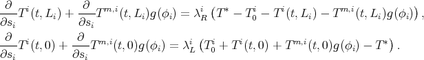
At the other end of each beam several obvious geometric compatibility conditions must be imposed. These conditions can be written in the form:
 (2.6) (2.6) |
In [1], system (2.1)-(2.6) was re-cast as an abstract second-order ODE in an appropriate Hilbert space. Semigroup theory was then used to prove that the system is well-posed. Moreover, it was shown that if Kelvin-Voigt damping to both transverse and longitudinal motions is added, then the corresponding semigroup is analytic and exponentially stable. The spectrum of the infinitesimal generator of this semigroup was also characterized. The case of local damping was analyzed in [4] where it was shown that if only one of the beams is damped, then only polynomial stability is obtained even if additional rotational damping is assumed in the joint. Numerical approximations and several numerical results are shown in [2].
The external heat flux in the space normal to the beam's surface is given by (see [10])
 (3.1) (3.1) |
where  denotes the solar flux and
  the angle of orientation of the solar vector with respect to the beam. In this equation we shall neglect the contribution of
  since we are assuming it is small. We denote by
  the deviation of the temperature of the thin-walled circular beam
  with respect to a reference temperature
  at time
  at the point on the beam corresponding to axial coordinate
  and circumferential coordinate
  (here
(here  corresponds to the top of the beam while
  corresponds to the bottom). Conservation of energy for a small segment of circular cylinder including longitudinal and circumferential conduction in the cylinder wall and radiation from the cylinder's surface yields the following equation for
  :
:
 (3.2) (3.2) |
where  and
and  are the axial and circumferential thermal conductivity coefficients, respectively,
  is the specific heat,
  the radius of the cylinder,
  is the thickness of the wall,
  is the surface emissivity and
  is the surface absorptivity,
  is the Stefan-Boltzmann constant,
  is a function defined on
 ![[- π, π]](/img/revistas/ruma/v49n2/2a0763x.png) by
by  for
for  , and
, and  for
for ![π π φi ∈ [- π,- 2 ] ∪ [2,π]](/img/revistas/ruma/v49n2/2a0767x.png) . The heat flux distribution on the RHS of equation (3.2) can be written as
. The heat flux distribution on the RHS of equation (3.2) can be written as
 (3.3) (3.3) |
where ![. 1 g(φi)= cos(φi)χ π π (φi) - π [-2 ,2]](/img/revistas/ruma/v49n2/2a0769x.png) (here
(here  denotes the characteristic function). Clearly
  is continuous and it has zero average in
 ![[- π,π]](/img/revistas/ruma/v49n2/2a0772x.png) .
.
For each beam, the temperature distribution is separated into two parts, namely:
 (3.4) (3.4) |
where  is independent of
  and corresponds to the uniform part of the flux,
  , in (3.3), and
  amounts for the circumferential variation of the flux in (3.3). Note that for every
 ![si ∈ [0,Li ]](/img/revistas/ruma/v49n2/2a0778x.png) and
and  one has that
  for any
 ![π π φ ∕∈ [- 2,2]](/img/revistas/ruma/v49n2/2a0781x.png) . Hence,
. Hence,  can be thought of as the thermal gradient between the top and the bottom of the beam at the axial location
  .
.
Also, we approximate the thermal radiation term 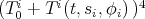 in (3.2) by linearizing
  around
  (where
  , to be determined later, is the steady-state constant temperature increment produced on the undeformed beam
  by the solar flux
  ), i.e., we approximate
 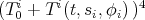 by
by  . Hence equation (3.2) is replaced by
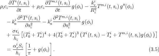
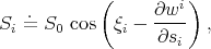
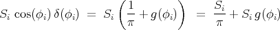
Since  has zero average, integration of equation (3.5) over the cylinder's cross sectional area yields
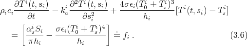
Since  is discontinuous at
  the integration of
  above must be performed in the distributional sense. The value of
  is now determined by setting the RHS,
  , equals to zero. By doing so we obtain
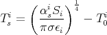 (3.7) (3.7) |
Note that with this value of  corresponds to the steady-state
 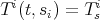 for the case of homogeneous Neumann boundary conditions and, since usually
  is small compared to
  , the linearization of the thermal radiation term performed above, is justified near the steady state solution.
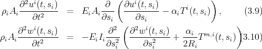
Now multiplying (3.5) by  and integrating over the cylinder's cross sectional area, we obtain for
  the following equation:
 (3.8) (3.8) |
Thermally induced vibrations in the system is taken into account by considering Hooke's law for the stress-strain relation in the form 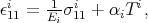 where
where  is the thermal expansion coefficient, and
  is, as before, the deviation from the reference temperature
  . Note that at
  thermal strain vanishes, so that
  is interpreted as the (uniform) temperature of beam
  in the unstressed, rest-state. By the standard derivation of Euler-Bernoulli beam equation, we modify the Joint-Leg-Beam system (2.1) as follows:
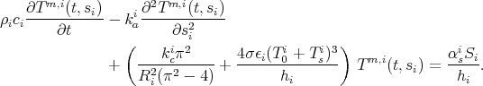
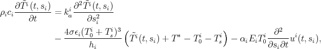
The above beam equations are coupled to the heat equations modified from equations (3.6) and (3.8) and with  chosen as in equation (3.7) (so that
  in (3.6) ), that is:
 (3.11) (3.11) |
and
![m,i 2 m,i [ i 2 i i3 ] ρc ∂T----(t,si) = ki ∂-T---(t,si)-- ---kcπ-----+ 4-σεi(T-0 +-T-s) T m,i(t,s ) ii ∂t a ∂s2i R2i(π2 - 4) hi i i 3 i + αiEiIiT0---∂---wi(t,si) + α-sSi, (3.12) 2RiAi ∂s2i∂t hi](/img/revistas/ruma/v49n2/2a07119x.png)
We impose Robin type boundary conditions for the temperature at both ends of each beam, i.e.

![∀t ≥ 0, φi ∈ [- π,π], i = 1,2](/img/revistas/ruma/v49n2/2a07121x.png) , where
, where  is the temperature of the surrounding medium and
  ,
,  ,
,  , are nonnegative constants. By writing
  in terms of the decomposition given in (3.4) these equations take the form:
Since these equations must hold for all ![φi ∈ [- π,π]](/img/revistas/ruma/v49n2/2a07128x.png) it follows that
it follows that
and
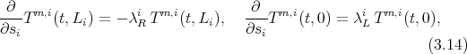
for all  ,
,  . So, in the same way that the dynamics for the temperature distribution (3.5) decouples into equations (3.11) and (3.12) for
  and
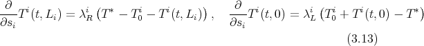
and  , respectively, we observe that the boundary conditions also decouple. Note however in equation (3.13) that the boundary conditions for the axial component of the temperature,
  , are non-homogeneous. By defining
  , equation (3.11) can be written in the form
 (3.15) (3.15) |
while the boundary conditions (3.13) now take the form

Observe now that these boundary conditions are exactly the same as those in (3.14) for the circumferential component of the temperature. Finally, note also that in equation (3.9),  can be replaced by
  without any changes.
System (3.9)-(3.12) (or equivalently (3.9), (3.10), (3.12), (3.15)), together with the joint-leg dynamics described by equation (2.2) constitute the thermoelastic Joint-Leg-Beam equations with the external solar heat source. The extensional forces, shear forces and bending moments of the beams at  are now given by:
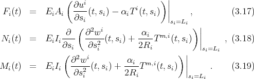
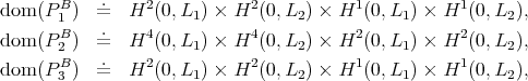
In this section, we consider the well-posedness of the Joint-Leg-Beam system with solar heat flux, i.e., equations (3.9), (3.10), (3.12), (3.15) subject to the geometric beam-leg interface compatibility conditions (2.6), the dynamic boundary conditions (3.17), (3.18), (3.19) and the boundary conditions (2.5), (3.14), (3.16). We first rewrite the system as a first order evolution equation in an appropriate Hilbert space. Well-posedness is then obtained by using semigroup theory. Since the corresponding system without thermal effects has been studied in [1], we will follow the notation used there as much as possible for consistency. Numerical results for that case are reported in [2].
First, we define the following Hilbert spaces with their corresponding inner products:
![( 2 2 2 2 |{ Hz = L (0,L1 ) ×2 L (0,L2) × L (0,L1 ) × L (0,L2), . ∑ [ i i i i ] |( ⟨z1,z2⟩Hz = ρiAi ⟨w1,w 2⟩ + ⟨u 1,u2⟩ ; i=1](/img/revistas/ruma/v49n2/2a07143x.png)
![{ Hb = [ker(C )]⊥ = range (CT ), ⟨b1,b2⟩H = ⟨b1,(CT M - 1C )†b2⟩lR6; b](/img/revistas/ruma/v49n2/2a07144x.png)
![( 2 2 2 2 |{ H ζ = L (0,L1 ) × L (0,L2) × L (0,L1 ) × L (0,L2), . ∑2 ρiciAi [ ] |( ⟨ζ1,ζ2⟩H ζ = ---i-- ⟨T m1,i,T m2,i⟩ + ⟨T˜1i,T˜i2⟩ ; i=1 T0](/img/revistas/ruma/v49n2/2a07145x.png)
where  , and
, and  denotes the Moore-Penrose generalized inverse of
  . We also define the operators
 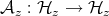 and
and 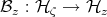 by
by
where  and for
  ,
,  denotes the space of functions in
  that vanish, together with all derivatives up to the order
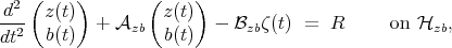
  , at the left boundary. With this notation, equations (3.9)-(3.10) can now be written as the following abstract second order ODE in
  :
:
 (4.1) (4.1) |
Next we define the operators 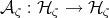 and
and 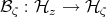 by
by
 |
![( [ ] ) ( ) - -k1a-D2T m,1 + ---k1cπ2----+ 4σε1(T01+T-1s)3- Tm,1 T m,1 | ρ1c12 [ρ1c1R212(π22-4) ρ1c1h21 23] | | T m,2| . || - -ka-D2T m,2 + ---kc2π-2---+ 4σε2(T0+T-s)- Tm,2|| A ζ ζ = A ζ|( T˜1 |) = || ρ2c2 k1 ρ2c2R2(π4-σ4ε1)(T1+T1ρ)23c2h2 || , ˜2 ( - ρ1ac1-D2 ˜T1 + ---ρ1c01h1s--˜T1 ) T - -k2a-D2 ˜T2 + 4σε2(T20+T2s)3˜T2 ρ2c2 ρ2c2h2](/img/revistas/ruma/v49n2/2a07163x.png) |
 |
 |
where  denotes the space of functions in
  satisfying the Robin boundary conditions (3.14) or equivalently (3.16). With this notation, equations (3.12), (3.15), can now be written as the following abstract first order ODE in
  :
:
 (4.2) (4.2) |
where
 |
We also define three boundary projection operators  ,
,  from
from  into
into  and
and  from
from  into
into  by
by
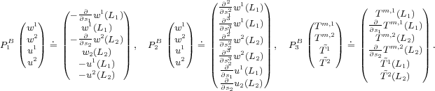
 :
:  (4.3) (4.3) |
where  ,
, 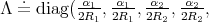
 and
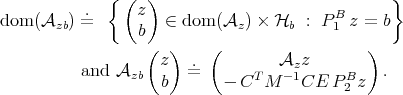
and  . Next we define the Hilbert space
 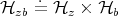 with the usual inner product inherited from those in
  and
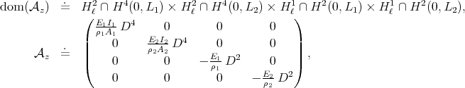
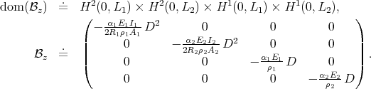
and  . In this Hilbert space we define the elastic operator
  by
by
 |
Furthermore, we define 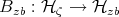 by
by  and
and 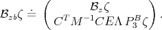 Thus, equations (4.1) and (4.3) can be combined as
 (4.4) (4.4) |
where  . It has been proved in [1] that the operator
  is self-adjoint and strictly positive. Thus, we can define the state space
 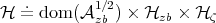 with the inner product
 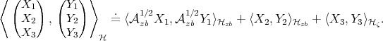 Finally, we define operator
  on
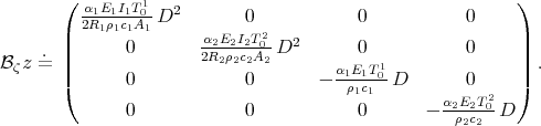
on  by
by 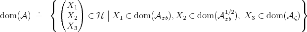 ,
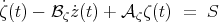
, 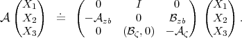 Then, equations (4.2) and (4.4) can be rewritten as a first order nonhomogeneous evolution equation
 (4.5) (4.5) |
where 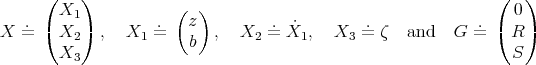 .
.
Theorem 4.1. (Well-posedness): Let  be as defined above. Then
  is the infinitesimal generator of a strongly continuous semigroup of contractions
  on
on  and hence, for any initial condition
 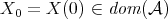 , system (4.5) has a unique global solution
  given by
Proof: It can be shown that  is dissipative and
  , the resolvent set of
  . Since
  is dense in
  , it then follows from Theorem 1.2.4 in [8] that
  generates a strongly continuous semigroup of contractions
  on
on  . The existence and uniqueness of solutions for system (4.5) for any initial condition
 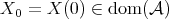 finally follows from Corollary 2.10 in [9]. For more details see [3]. _
We now turn our attention to the stability of system (4.5). It is well known that the semigroup associated with longitudinal and transversal motion of a thermoelastic Euler beam is exponentially stable ([5], [8]). System (4.5) consists of two thermoelastic beam equations plus the equations for the joint-leg dynamics. This type of system is often referred to as "hybrid system". It is certainly an interesting problem to determine whether the thermal damping is strong enough by itself to induce exponential stability of this kind of system. We shall prove this in the affirmative.
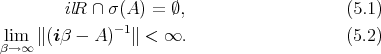
The following result by Huang [6] will be used:
Theorem 5.1. Let  be a Hilbert space,
  a closed, densely defined linear operator. Assume that
  generates a
  -semigroup of contractions
  on
on  . Then
  is exponentially stable if and only if
Theorem 5.2. The  -semigroup of contractions
  generated by
  (see Theorem 4.1) is exponentially stable.
Proof: If (5.2) is false then there exists a sequence  with
with  and a sequence
  with
with 
 such that
 (5.3) (5.3) |
Using the components related to the thermoelastic beam equations it can be show that (5.3) yields the contradiction  as
as  . Similarly, if the condition (5.1) is false, then there exist
  and a sequence
  with
with  , such that
 (5.4) (5.4) |
By repeating the same arguments we get the contradiction  . For complete details on these proofs, we refer the reader to [3]. Hence
  satisfies conditions (5.1) and (5.2) and therefore, the
  -semigroup of contractions
  generated by
  is exponentially stable. __
In this article we considered a system of two thermoelastic Euler-Bernoulli beams coupled to a joint through two legs. By means of semigroup theory the well posedness of the system was proved and its exponential stability was derived. It is certainly of much interest to develop numerical approximations for our state-space model (4.5). Such numerical schemes will be useful in simulation and identification studies to predict and better understand the structural and thermal responses of space-borne observation systems. Efforts in this direction are already under way.
This work was supported by DARPA/SPO, NASA LaRC and the National Institute of Aerospace under grant VT-03-1, 2535, and in part by AFOSR Grants F49620-03-1-0243 and FA9550-07-1-0273. Acknowledgement is also given to CONICET and Universidad Nacional del Litoral of Argentina.
[1] J.A. Burns, E.M. Cliff, Z. Liu and R. D. Spies, On Coupled Transversal and Axial Motions of Two Beams with a Joint, Journal of Mathematical Analysis and Applications, Vol. 339, 2008, pp 182-196. [ Links ]
[2] J.A. Burns, E.M. Cliff, Z. Liu and R. D. Spies, Results on Transversal and Axial Motions of a System of Two Beams coupled to a Joint through Two Legs, submitted, 2008. ICAM Report 20070213-1. [ Links ]
[3] E.M. Cliff, B. Fulton, T. Herdman, Z. Liu and R. D. Spies, Well posedness and exponential stability of a thermoelastic joint-leg-beam system with Robin boundary conditions, Mathematical and Computer Modelling (2008), en prensa, DOI: 10.1016/j.mcm.2008.03.018. [ Links ]
[4] J.A. Burns, E.M. Cliff, Z. Liu and R. D. Spies, Polynomial stability of a joint-leg-beam system with local damping, Mathematical and Computer Modelling, Vol. 46, 2007, pp 1236-1246. [ Links ]
[5] J.A. Burns, Z. Liu and S. Zheng, On the Energy Decay of a Linear Thermoelastic Bar. J. of Math. Anal. Appl., Vol. 179, No. 2, 1993, pp 574-591. [ Links ]
[6] F. L. Huang, Characteristic Condition for Exponential Stability of Linear Dynamical Systems in Hilbert Spaces, Ann. of Diff. Eqs., 1(1), 1985, pp 43-56. [ Links ]
[7] C. H. M. Jenkins (ed.), Gossamer Spacecraft: Membrane and Inflatable Technology for Space Applications, AIAA Progress in Aeronautics and Astronautics, (191), 2001. [ Links ]
[8] Z. Liu and S. Zheng, Semigroups Associated with Dissipative Systems, 398 Research Notes in Mathematics, Chapman & Hall/CRC, 1999. [ Links ]
[9] A. Pazy, Semigroups of Linear Operators and Applications to Partial Differential Equations, Second Edition, Springer Verlag, 1983. [ Links ]
[10] E. A. Thornton and R. S. Foster, Dynamic Response of Rapidly Heated Space Structures. In: Computational Nonlinear Mechanics in Aerospace Engineering, edited by Atluri, S.N., Progress in Astronautics and Aeronautics, Vol. 146, AIAA, Washington D.C., 1992, p. 451-477. [ Links ]
E. M. Cliff
Interdisciplinary Center for Applied Mathematics
Virginia Polytechnic Institute and State University
Blacksburg, VA, 24061-0531, USA.
Z. Liu
Department of Mathematics
University of Minnesota
Duluth, MN 55812-3000, USA.
R. D. Spies
Instituto de Matemática Aplicada del Litoral
IMAL, CONICET-UNL, Güemes 3450, and
Departamento de Matemática,
Facultad de Ingeniería Química, UNL,
Santa Fe, Argentina
rspies@imalpde.santafe-conicet.gov.ar
Recibido: 11 de mayo de 2008
Aceptado: 20 de mayo de 2008

