


Servicios Personalizados
Revista

Articulo
 Inglés (pdf)
 Articulo en XML
 Referencias del artículo
 Enviar articulo por email
Indicadores
-
 Citado por SciELO
Links relacionados
-
 Similares en
SciELO
Similares en
SciELO
Compartir

 Permalink
Latin American applied research
versión impresa ISSN 0327-0793
Lat. Am. appl. res. v.33 n.4 Bahía Blanca oct./dic. 2003
Groebner bases for designing dynamical systems
G. L. Calandrini1,3, E. E. Paolini and J. L. Moiola2,3
Departamento de Ingeniería Eléctrica, Universidad Nacional del Sur Avda. Alem 1253 (8000) Bahía Blanca - Argentina
calandri@criba.edu.ar
1 Departamento de Matemática, Universidad Nacional del Sur
2 Mathematical Institute, University of Cologne, 50931 Cologne, Germany
3 CONICET (Consejo Nacional de Investigaciones Científicas y Técnicas)
Abstract ¾ The design or synthesis of systems exhibiting a prescribed trajectory is presented in this paper. The design process is based on algebraic concepts, and it relies heavily on the use of Groebner bases. It is assumed that both the trajectory and its dynamics can be represented as algebraic relationships between the variables of the system and their first derivatives. The method yields a dynamical systems with the desired behavior as one of its many solutions.
Keywords ¾ Groebner Bases. Control Theory. Dynamical Systems. Differential Equations.
I. INTRODUCTION
Over the last years, a great progress has been performed in the field of differential equations through the study of the different dynamical configurations obtained when varying some parameters of the system. hi this field, one of the most promising results is the representation of certain dynamic phenomena using an elementary form, with polynomial-type relationships among their variables, the normal form. This representation describes the typical effects in the simplest way not only among the main variables (normal form) but also its parameters (unfoldings), after making a series of transformations on the original system.
The normal form and its unfoldings in the parameter space explains the elementary dynamics exhibited by the system, and this model is still valid for certain perturbations in higher order terms (i.e., relationships between polynomials of higher order). Synthesizing dynamical systems by means of normal forms became feasible with the appearance of algebraic symbolic algorithms, contributing to study the system dynamics in an analytic way. Although in the majority of the nonlinear systems it is not possible to find explicit solutions, except through the use of numerical methods, these techniques are still very powerful for validating the results.
Advances in computer technology and the availability of software packages to perform symbolic mathematics, like Mathematica, Maple, Reduce, etc. stimulated the study of some theories and techniques developed previously, particularly the concept of Groebner bases, formulated by Buchberger in 1965. (A brief review of the algebraic concepts used through the paper is contained in the Appendix.) Buchberger proved the fundamental theorems on which the theory is based and proposed an algorithm to compute such bases (Buchberger, 1965, 1970, 1995). The advent of specialized software for computational algebra (CoCoA, Macaulay and Singular, etc.) expanded the studies of computational algebra to other fields, for example dynamical systems and control theory (Forsman, 1995; Fortell, 1995; Jirstrand, 1996; Alwash, 1996, among others).
The design of dynamical systems exhibiting a prescribed orbit as one of its solutions is explored in this paper. The design process consists in finding a differential system from the specification of the desired orbit and its dynamical behavior by means of Groebner bases. It seems that normal forms -a polynomial characterization of the system dynamics- and Groebner bases will develop profound connections in a near future. In this vein, this paper constitutes a first step in enlightening some preliminary applications of synthesis of nonlinear systems using Groebner bases.
II. OBJECTIVE
The synthesis process developed in this paper aims at designing a system  with an a priori chosen solution x = xd(t), and also endowing this solution with asymptotically orbital stability. The proposed solution defines a trajectory or orbit, i.e. the image g of xd(t) in the state-space,

This set is positively invariant, and the dynamical behavior of the solution is determined by the restriction of f(.) onto the set g, given by the time derivative of the solution  . In other words, we will impose that every solution with an initial condition in g, remains in it for all t ³ 0. We will also require
that the proposed orbit g has asymptotic stability, i. e. that every solution x(t) remains in an arbitrarily small e-neighborhood of g for any initial condition inside a d-neighborhood, and that the distance between x(t) and the set g tends to zero as t tends to infinity.
There are many possibilities for specifying invariant sets and dynamical behavior. One way is through the explicit temporal parameterization of the solution. Although this approach facilitates the specification of the desired orbit, it is not adequate for design purposes. For this reason, a different approach will be adopted here. Following Berns et al. (2001) it is possible to eliminate the variable t from a polynomial set determined by xd(t) and  to obtain another polynomial set with certain properties, known as Groebner basis. Therefore, the desired invariant set and its dynamics are replaced by a specification more akin to design: a Groebner basis. This mathematical tool has been used previously for the study of the dynamical systems by Alwash (1996) in order to determine multiple limit cycles in polynomial systems and, more recently, by the authors for the synthesis of oscillators (Berns et al., 2001), but without analyzing the stability of the solutions.
III. DYNAMICAL SYSTEMS WITH POLYNOMIAL IDEALS
Let us consider the autonomous system represented by the classical state-space description
 | (1) |
where f1, ..., fn ¬ k[x1, ..., xn] are polynomials in the variables x1, ..., xn, with coefficients in the field k, being k either  ,
,  , or the field of rational functions of parameters of the system. This representation comprises a large class of systems including many nonlinearities, like trigonometric functions, that although are not polynomial functions can be expressed as solutions of algebraic-differential equations (Fliess, 1990). Therefore in the following, it will be assumed that polynomials f1, ..., fn in (1) not only represents the classical state-space description, but also the algebraic-differential equations necessary to include non-polynomial terms of the class described above.
From an algebraic perspective, dynamical systems can be studied as algebraic relationships between the state variables and their first derivatives. We will assume that the set of state variables is algebraically independent, i.e. that no polynomial p Î k[x1, ..., xn] vanishes when the variables take values over any trajectory or solution of the system. However, the inclusion of an additional variable, for example the first time derivative  of the state variable xi, renders this new set algebraically dependent, i.e. there is at least a polynomial p Î
  such that p((t), x1(t), ..., xn(t)) = 0 for any solution of the system. Therefore, from an algebraic viewpoint, a system can be denned as the set of every polynomial p belonging to the ring that identically vanishes when the variables take values over every solution trajectory of the system under consideration. This infinite polynomial set is an ideal, and Hubert's theorem on basis assures that it can be characterized with a finite generating set. Although this viewpoint embraces a large class of algebraic systems, we will only consider those equivalent to the classical state-space representation.
The set  vanishes over every solution of (1), and the same happens with every polynomial of the ideal generated by this set.
Definition. Given an algebraic-differential description (1) of a system, the ideal of the system associated to this description is the ideal X generated by the set S = , noted as  .
.
In other words, the polynomials of the algebraic-differential equations (1) constitute a generating set of the ideal of the system. After fixing a monomial ordering1, every ideal has a unique reduced Groebner basis (Cox et al., 1992). Furthermore, if G is a Groebner basis of an ideal, a polynomial f belongs to the ideal if and only if the remainder of the division of f by G is zero. This means that a Groebner basis is a very appropriate generating set to identify an ideal because (i) it is unique and (ii) it suffices to compute a division remainder to ascertain if a polynomial belongs or not to the ideal.
Notice that, depending of the realization, sometimes it is convenient to consider that the ideal of the system is generated either in the ring (i.e., the ring of polynomials in the variables  and coefficients in the field k) or in the ring k(x1, ..., xn)[
 ] (i.e., the ring of the polynomials in and coefficients in the field of rational functions in x1, ...,xn with coefficients in k). Now let us consider the first case and the ordering of the variables
  and the lexicographical monomial ordering (Lex). The polynomials of S are linear in , i = l, ..., n, and according to the chosen ordering, the terms containing these variables are also the leading monomials. Therefore they generate every leading monomial of the polynomials of S. Then, S is a Groebner basis of S, and due to the linearity of the leading monomials, the polynomials of S are irreducible, implying that the ideal S is prime. In consequence, it is also radical meaning that it contains all the polynomials of the ring vanishing at the same solutions than the set S.
On the other hand, the independence of the state variables implies that  and thus S is also the Groebner basis of
  , the ideal generated by S in the ring k(x1, ...,xn)[], corresponding to the Lex ordering with
  , where the coefficients are rational functions in the state variables.
A. Invariant sets
To specify invariant sets, we make use of affine varieties defined on the state-space: the set of every solutions of a system of polynomial equations p1= p2 = ... = ps = 0, with pi Î k[x1, ...,xn]. In other words, there exists an algebraic dependence between the state variables given by these polynomials. The set defined by the affine variety in the state-space will be noted as V(I), where I is the polynomial set described by the system of equations I = {p1,p2, ...,ps}. A set V(I) is invariant with respect to a system S if it verifies dpi / dt = 0 for all t ³ 0. In other words, the polynomials

must belong to the ideal of the system S restricted to V(I).
Let V(I) be an invariant set with respect to the system . The restriction of the dynamics to the invariant set can be studied from the ideal generated by I È S. This dynamics can be characterized by a Groebner basis SI for  , that has a particular structure when using the ordering , and can be written as SI = Gx È Gd. The set of polynomials Gx = SI Ç k[x1, ..., xn] is an implicit expression of the invariant set defined by the affine variety V(I). The set of polynomials Gd, also containing polynomials depending linearly on the first derivative of the state variables, defines the dynamics over the invariant set V(I) (the restriction of the dynamics S over the invariant set V(I)).
B. Stability of invariant sets
Lyapunov stability theory and LaSalle's theorem in particular (Khalil, 1996), can be used to address the stability of invariant sets.
Theorem (LaSalle): Let W Ì D be a compact set, positively invariant with respect to (1). Let V : D ® R be a continuously differentiable function such that  in W. Let E be the set of every point in W where
  . Let M be the largest invariant set contained in E. Then every solution starting in W approaches M as t ® ¥.
This theorem does not require the positive definite-ness of function V(x). Furthermore, the set fi needs not to be related to V(x). However, V(x) can be constructed to guarantee the existence of the set W. In particular if  is a bounded region and V(x) £ 0 for all x Î Wc, then it can be chosen W = Wc.
IV. SYNTHESIS PROCEDURE
The starting point for the synthesis procedure is a given invariant set (i.e. the desired trajectory represented by a polynomial set Gx) and the desired dynamic behavior of the solutions over it given in implicit form by a polynomial set Gd. The union of these two sets forms a Groebner basis SI = Gx È Gd. Let

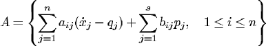
where pj, qi Î k[x1, ..., xn], j = l,...,s, i = l, ..., n. This basis generates an ideal of polynomials SI; the polynomials in this ideal are expressions of several dynamical relationships among the variables, corresponding to different state equations that have the desired orbit as one of their many possible solutions.
The objective of this paper is to design a system with this orbit as a solution, having the property of being a stable limit set of the system: all the trajectories beginning in a neighborhood of the orbit will approach it as time t tends to infinity. Therefore, the polynomials defining the system with the proposed orbit are in the ideal SI, i.e. they are combinations of the polynomials of SI. To be more specific, let us consider the following n combinations of polynomials

where aij and bij are polynomials in the ring k[x1, ..., xn].
The set A is included in k(aij, bij, x1, ..., xn)[]. The designed system can be represented by a Groebner basis S,  guaranteeing at the same time the algebraic independence of these combinations.
If the leading coefficients of this basis do not vanish simultaneously2, the n polynomials of the set S are algebraically independent. Therefore, polynomials aij and bij must be chosen to fulfill this requirement. A closer look reveals that another set of requirements on aij, bij can be imposed from the specification of the behavior of the system in the exterior of the orbit. With this objective in mind, we build up a positive semidefinite function such that it vanishes on the orbit and it is positive in the rest of the state-space. One of such functions is the polynomial

in the ring k[x1, ...,xn], because it has a minimum on the orbit, and the minimum value is zero. In order to apply LaSalle's theorem,  has to be negative semi-definite and thus the dynamics of V has to be chosen accordingly. Clearly
  will be zero at those points where any of the following conditions are verified: (i) the gradient of V is zero, (ii) the gradient is normal to the trajectory, (iii) the points are equilibrium points. For design purposes, cases (ii) and (iii) must be avoided because they reduce the basin of attraction of the prescribed orbit. With respect to the case (i), clearly the gradient is zero over the orbit V = 0; the other points where the gradient vanishes may be found considering the set of polynomials

composed by the components of the gradient and an additional polynomial zV - 1 in the auxiliary variable z. If {g1, ..., gm} is the Groebner basis for  , where the monomial ordering is chosen to eliminate the auxiliary variable z, the zero set of these polynomials comprises only the points where the gradient vanishes and excludes any point of the orbit V = 0, because the inclusion of the polynomial zV - 1 in P implies V Ï . Therefore, the dynamics for V can be written as
 (2)
(2)
where a is a positive polynomial. To simplify the exposition we will consider the case when a is a zero-order polynomial, i.e. 0 < a Îk, a positive design parameter. Then the function is negative semidefinite, and takes the zero value in those points where the gradient is zero. Of course, this election for is entirely arbitrary, and other possible options are for example  , where ai are arbitrary positive polynomials, or
 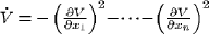 .
.
The polynomial

which captures the dynamics of the system must belong to the ideal S Ì k(ak, aij, bij, x1, ..., xn) []. Since S is a Groebner basis for S, the remainder of p with respect to S must be zero. The zeroing of the remainder reveals the algebraic relationships between the unknown coefficients aijand bij. As stated before, they must be properly chosen such that (i) the remainder is zero, and (ii) no leading coefficients of S vanishes. This concludes the design of the system S, generated by the Groebner basis S.
Orbital stability analysis. The analysis of the orbital stability can be performed by means of LaSalle's theorem. As by design in the whole state-space [see (2)], to fulfill the remaining hypothesis two sets Wc and E have to be defined, such that (i)  is bounded for a certain value c to be found, and (ii) the set E (the set of all points in W where ) coincides with the points of the desired orbit, i.e. E = M = g.
The first issue is addressed noticing that, given a bounded orbit, it is always possible to find a value c (albeit small) such that Wc is bounded because V is a continuous positive function that takes the zero value on a compact set (the orbit g). To guarantee that E = g, it is necessary to prove that if another solution exists for which it has to be isolated of g. In this way, the orbit is the only invariant set in E to which every solution starting in Wc approaches to g as t tends to infinity.
A. Summary of the synthesis procedure
Step 1. Express the specifications with the polynomial set SI = Gx È Gd where SI is a Groebner basis and

with pi, qi Î k[x1,...,xn].
Step 2. Build up the set
and find the Groebner basis S for  in the ring
Step 3. Build up the positive semidefinite function
Step 4. Find the Groebner basis {g1, ..., gm} of the z-elimination ideal (z > x1 > ... > xn) generated by  , in the ring k[x1, ..., xn], i.e.,
  , and choose a suitable V (e.g.
  ).
).
Step 5. Compute the remainder of the polynomial  with respect to S in the ring k(ak,aij, bij, x1, ..., xn)[].
Step 6. Choose the coefficients aij and bij so that the remainder is zero.
Step 7. Select the ideal generated by S as the designed system.
Step 8. If the desired orbit is not bounded, check out the orbital stability.

Figure 1: Positive semidefinite function V(r, z).

Figure 2: Temporal derivative of the function V, with r1 = 1, and r2 = 0.5.
V. EXAMPLES
A. Torus-type orbit
As an example of the technique discussed above, we propose the design of a system that has a torus-type orbit. The torus is described in cylindrical coordinates. The state variables are r, q and z, with x = rcosq and y = rsinq. To simplify the design, it is assumed that the angle q is not involved in the dynamics of the other two variables, and that the dynamics of the rotation is fixed ( = w = constant) restricting the design to the r-z plane, where the torus describes a circle centered in r = r1 and z = 0, with a radius r2, 0 < r2 < r1 and rotating at a constant angular speed w2.
Step 1. The desired orbit is given by  . Thus the invariant set and its dynamics are defined by the set of polynomials SI = Gx È Gd,

Step 2. Let us define the field k = (a, r1, r2, w1, w2).
The combination of the polynomials of SI in the ring  gives the generating set of the ideal of the system to be designed

where a,b,c,d Î k[r, z]. The Groebner basis S for in the ring 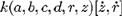 corresponding to the ordering
  is given by

where 1 - bd ¹ 0 to guarantee that the chosen combination of polynomials is algebraically independent.
Step 3. The function defining the dynamics outside of the orbit is chosen as  . A plot of this function is shown in Fig. 1 revealing that it is positive semidefinite on the plane r-z, and vanishes on the orbit g.
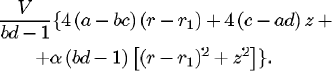
Step 4. The gradient of this function vanishes on the orbit, and also in the variety defined by the set of polynomials {r - r1, z}. With these polynomials it is possible to fix the dynamics in the exterior of the orbit making = -aV[(r - r1)2 + z2]. Figure 2 shows that is zero on the orbit and also in the center of the circle.
Step 5. The remainder of  with respect to S is
Step 6. This polynomial is in  , and it is zero over g, and also over the rest of the r-z plane if
  .
.
Step 7. Replacing these values in S, the Groebner basis for the designed system is found to be

Step 8. For the stability analysis of the orbit, clearly the set  is compact, and choosing
  , the orbit g is the only invariant contained in Wc where .

Figure 3: Temporal evolution of the Cartesian variables in the designed system.

Figure 4: Torus orbit of the designed system.
Therefore, according to LaSalle's theorem, the orbit is asymptotically stable.
It is worth noting that the dynamics in the r-z plane corresponds to the normal form of a stable cycle of radius r2. The description of the system with a torus-type orbit in cylindrical coordinates is given by
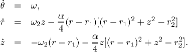
Figure 3 shows the temporal evolution of the Cartesian variables x, y, z, for r1 = 1, r2 = 0.5, w1 = 1, w2 = 0.5, and a = 0.5, and the initial conditions r(0) = 1, z(0) = 0.01 and q(0) = 0. The torus orbit in the state-space is shown in Fig. 4.
B. A limit cycle
In this example the invariant set is a limit cycle defined by the affine variety p1 = 0 in  where
where  . The desired orbit is then given by
  .
.
Step 1. The invariant set and its dynamics are represented by the set of polynomials SI = Gx È Gd, where Gx = {p1}, Gd = {q1,q2}, with  ,
,  .
.
The invariant set may be checked performing the quotient between the polynomial  with respect to SI = {p1, q1, q2}. Clearly,
  , meaning that the remainder is zero, and thus
  .
.
Step 2. The combination of the polynomials of SI in the ring (x1,x2) gives the generating set of the ideal of the system to be designed

where a,b Î [x1,x2]. The Groebner basis S for in the ring (a, b, x1, x2), corresponding to the ordering  is given by S = A.
Step 3. The function defining the dynamics outside of the orbit is  .
.
Step 4. The gradient of this function vanishes on the orbit, and also in the variety defined by the set of polynomials {x1, x2 + 1}. However, we fix the dynamics in the exterior of the orbit choosing  .
.
Step 5. The remainder of  with respect to S is

Step 6. This polynomial is in (a, b, x1 x2) and is zero over g, and also over the rest of the x1-x2 plane if  ,
,  .
.
Step 7. Replacing these values in S, a Groebner basis for the designed system is obtained. This can be written as the following state-space equations

Step 8. To determine the stability of the orbit, clearly the set  is compact, for a small c value, due to the continuity of V and the boundness of the orbit. Furthermore, the orbit g is the only invariant contained in Wc where . According to LaSalle's theorem, the orbit is asymptotically stable. Figure 5 shows simulation results that confirm this fact, even for small values of parameter a (a = 5 ´ 10-7) that sets how fast the trajectories approach to the desired orbit.

Figure 5: Limit cycle of the designed system.
VI. CONCLUSIONS
In this paper, a constructive procedure for designing systems with prescribed orbits has been presented. An algebraic viewpoint seems appropriate for this purpose, and the main tool is an algorithm to compute Groebner basis of polynomial ideals. This algorithm is already available in software performing symbolic calculus, like Mathematica, Maple, etc. or more specific environments such as Macaulay and CoCoA. The application of the method is shown with the design of a system with a torus-type orbit and a specified limit cycle. The procedure presented here is the first step toward the synthesis of normal forms of systems containing certain specified dynamics.
VII. APPENDIX
We resume in this appendix some basic algebraic concepts. In the following, R = k[x1, ..., xn] is the ring of polynomials in x1, ..., xn with coefficients in a field k. The interested reader should consult (Cox et al., 1992) or (Kreuzer and Robbiano, 2000) for more details.
1. A subset I Ì k[x1, ... ,xn] is an ideal if it satisfies (i) 0 Î I; (ii) If f, g Î I then f + g Î I; (iii) If f Î I and h Î k[x1, ... , xn], then h f Î I.
2. A natural way of defining ideals is using a finite polynomial set. Let f1, ..., fs Î R. The set  is an ideal, and it is called the ideal generated by f1, ..., fs.
3. A polynomial f Î R is irreducible over k if f is nonconstant and it is not the product of two nonconstant polynomials in R.
4. An ideal I Ì R is said to be prime if whenever the product f × g belongs to I, either f Î I, or g Î I (or both).
5. Let I Ì R be an ideal. An ideal I is said to be radical if gm Î I, for any integer m ³ 1 implies that g Î I.
6. The solutions of polynomial equations can be curves, surfaces, or objects of greater dimension, denominated affine varieties. The affine variety V denned by the polynomials f1, ..., fs is the set  , i.e. the set of all the solutions of the system of equations f1 = ... = fs = 0.
7. Let V Ì kn be an affine variety. Then, the set  , the set of all the polynomials vanishing on the given variety is an ideal and it is radical. The strong Nulstellensatz's theorem proves that if k is an algebraically closed field, and I a radical ideal in k[x1, ..., xn], then I(V(I)) = I, i.e. it exists a one-to-one correspondence between affine varieties and radical ideals.
8. The Hubert Basis Theorem (Cox et al., 1992) proves that every ideal in R has a finite basis. The Groebner bases constitute a special type of generating set of polynomial ideals and one of their properties is to eliminate variables in systems of polynomial equations. Starting from a finite generating set, the algorithm devised by Buchberger (1970) allows to calculate a Groebner basis for any ideal. In order to apply the algorithm, it is necessary to define the ordering of the variables and also the ordering of the terms of the polynomials or monomials; the algorithm tries to eliminate the higher order variables. If a = (a1, ..., an) and b = (b1, ..., bn) Î  are two vectors of exponents, according to the Lexicographical (Lex) order, a <Lex b if and only if
  and
and  .
.
9. Once a monomial ordering is chosen, the terms of a polynomial can be ordered without ambiguity. The maximum monomial of a polynomial f is denominated leading monomial LM(f); its coefficient (not null) is the leading coefficient LC(f), and the leading term is the product of both, LT(f) = LC(f) × LM(f).
10. A finite subset G = {g1, ..., gs} of an ideal I is a Groebner basis if  . This means that a set {g1, ..., gs} Ì I is a Groebner basis of I if and only if the leading term of every polynomial in I is divisible for one of the LT(gi).
11. It is possible to carry out "quotients" in the ring R with an algorithm. One could divide a polynomial f by a polynomial set {f1, ..., fs} Ì R and express f with the combination f = a1f1 + ... + asfs + r where the quotients ai and the remainder r belong to R. Let G be a Groebner basis of an ideal I. Then f Î I if and only if the remainder of the division of f by G is zero.
1 For the reader not familiarized with algebraic concepts, a brief review is given in the Appendix.
2 Although the leading coefficient in the reduced bases is always 1, when "working in the field of rational functions with symbolic mathematical software (e.g, Mathematica, Maple, etc.) it is sometimes convenient to multiply the polynomials by a leading coefficient being the minimum common multiple of all the denominators of the rational functions acting as coefficients of the polynomials. In this way, the software packages work with polynomial (and not rational) coefficients; at present time, this allows a faster and less intensive computation of the bases.
ACKNOWLEDGMENT
J.L.M. acknowledges the support received by the Alexander von Humboldt Foundation.
REFERENCES
1. Alwash, M. A. M., "Periodic solutions of a quartic differential equation and Groebner bases", J. Comput. Appl. Math. 75, (1), 67-76, (1996). [ Links ]
2. Berns, D. W., G. L. Calandrini, E. E. Paolini and J. L. Moiola, "Synthesis of nonlinear oscillators using Groebner bases", in Proc. Workshop on Nonl. Dynam. of Electr. Systems (NDES2001), 85-88, Delft, The Netherlands, (2001). [ Links ]
3. Buchberger, B. "Ein Algorithmus zum Auffinden der Basiselemente des Restklassenringes nach einem nulldimensionalen Polynomideal", PhD. thesis, Math. Inst. Univ. of Innsbruck, Austria (1965). [ Links ]
4. Buchberger, B. "Ein algorithmisches Kriterrum fur die Losbarkeiteines algebraischen Gleichungsystems", Aequationes Mathematicae 4, 374-383, (1970). [ Links ]
5. Buchberger, B. "Introduction to Groebner bases", Logic of Computation, Marktoberdorf, 35-66, (1995). [ Links ]
6. Cox, D., J. Little and D. O'Shea, Ideals, Varieties and Algorithms: An Introduction to Computational Algebraic Geometry and Commutative Algebra, Undergraduate Texts in Mathematics, Springer, (1992). [ Links ]
7. Fliess, M. "Generalized controller canonical forms for linear and nonlinear dynamics", IEEE Trans, Aut. Control 35, 9, 994-1001, (1990). [ Links ]
8. Forsman, K. "Elementary aspects of constructive commutative Algebra", PhD. thesis, Depart. of Electr. Engng. Linköping University, Linköping, Sweden, (1995). [ Links ]
9. Fortell, H. "Algebraic approach to normal forms and zero dynamics", Technical Report, Depart. of Electr. Engng. Linköping University, Linköping, Sweden, (1995). [ Links ]
10. Jirstrand, M. "Algebraic methods for modeling and design in control", PhD. thesis, Depart. of Electr. Engng. Linköping University, Linköping, Sweden, (1996). [ Links ]
11. Khalil, H. K., Nonlinear Systems, 2nd. Edition, Prentice Hall, (1996). [ Links ]
12. Kreuzer, M., and L. Robbiano, Computational Commutative Algebra 1, Springer, (2000). [ Links ]

