Robust identification of PWL-Wiener Models: use in model predictive control

A. Lusson Cervantes, O.E. Agamennoni and J.L. Figueroa¹

Dpto. de Ingeniería Eléctrica y de Computadoras, Universidad Nacional del Sur
Avda. Alem 1253, 8000 - Bahía Blanca, Argentina
alusson@criba.edu.ar iegamenn@criba.edu.ar
¹ also in Planta Piloto de Ingeniería Química, (PLAPIQUI - UNS - CONICET),
jfigueroa@plapiqui.edu.ar

Abstract ¾ In this paper a robust identification strategy for Wiener like models constituted by a linear dynamic block in series with a Piecewise Linear (PWL) function as the nonlinear static gain is presented. The proposed realization allows straightforward characterization of the static gain uncertainty. A robust Model Predictive Control (MPC) algorithm, using the presented modeling strategy, is developed to guarantee that no constraints in the feedback loop are violated.

Keywords ¾ Identification. Wiener Model. Robustness. Model Predictive Control.

I. INTRODUCTION

In the last years, several approaches to incorporate nonlinearities in to controller design strategies have been presented. In particular, the Wiener like models deserve attention as they are suitable for the description of systems which are internally linear but have a static nonlinear output transformation (e.g. pH neutralization processes). They can also be used for the approximation of nonlinear fading memory systems (Castro et al., 1999). Most of the dynamical systems in industry belong to this class of nonlinear systems. The choice of Wiener models in control was also motivated by recent results on nonlinear system identification (Westwick and Verhaegen, 1996) and by their straightforward applications in nonlinear Model Predictive Control. Important results in this field can be found in Norquay et al., (1998, 1999a) and in Gerksic et al. (2000). Moreover, some practical implementations of these algorithms have been reported by Norquay et al., (1999b).

Model predictive control (MPC) refers to a class of computer control algorithms that control the future behavior of a plant through the use of an explicit process model. At each control interval, the MPC algorithm computes an open-loop sequence of manipulated variable adjustments in order to optimize the future plant output. The first input in the optimal sequence is injected into the plant, and the entire optimization is repeated at subsequent control intervals (Qin and Badgwell, 1997).

Though manufacturing processes are inherently nonlinear, the vast majority of MPC applications up to date are based on linear dynamic models, the most common being step and impulse response models derived from the convolution integral. There are several potential reasons for this, for example; by using a linear model and a quadratic objective, the nominal MPC algorithm takes the form of a highly structured convex Quadratic Program (QP), for which reliable solution algorithms and software can easily be found. The algorithm solution must converge reliably to the optimum value in no more than a few tenths of a second to be useful in industrial applications. This is the reason why linear MPC is widely preferred over the nonlinear version.

Nevertheless, there are cases where nonlinear effects are significant enough to justify the use of Nonlinear Model Predictive Control (NMPC). With the introduction of a dynamic nonlinear model within the NMPC algorithm, the complexity of the predictive control problem increases significantly. Review papers by Bequette (1991) and Henson (1998) study the various approaches to handle nonlinear systems via MPC. In particular, the Wiener models (Norquay et al., 1998, 1999a, 1999b; Gerksic et al., 2000) have a special structure that facilitates their application to NMPC.

In this paper a particular realization for the Wiener model, where the static gain is described by a Piecewise Linear function (PWL) is presented. These PWL functions have proved to be a very powerful tool in the modeling and analysis of nonlinear systems. The PWL Functions are used since 1965 in the area of nonlinear circuit theory. In the 70's, they are specially relevant in the works of Leon Chua (1971) where the treatment of systems in is properly solved. But only recently with the work of Julián et al. (1999) on High Level (HL) PWL it is possible to obtain expressions to solve the general problems in . These expressions allow the development of a systematic and uniform approximation of any continuous nonlinear function in a compact domain.

Here, we present a strategy to identify Wiener models with PWL functions representing the nonlinear gain. In particular, an uncertainty description will be incorporated into the static nonlinearity as gain bounds. A robust Wiener Model Predictive Control (WMPC) will be presented to guarantee that, in the presence of model uncertainties, no constraints in the feedback loop are violated. It is assumed that the function f of the system under control is biyective, i.e. it has an inverse. This is a reasonable assumption for a large set of process models. Then, the PWL function used for the approximation will have an inverse too, and a simple set point transformation allows the formulation of the nonlinear MPC problem as a linear MPC.

The paper is organized as follows; in Section II a description of the Wiener model is presented, stressing the use of the PWL functions to represent the static nonlinearity. In Section III a methodology to approximate a PWL function and uncertainty bounds is discussed. The model identification is described in Section IV. In Section V, the WMPC is defined in face of the identified model. The proposed methodology is applied in Section VI to a neutralization reactor, and finally, the Conclusions are included in Section VII.

II. WIENER MODELS

In this work, a Wiener approximation will be used to represent the model process. In general, a Wiener model consists of a dynamic linear block (H1) in cascade with a static nonlinearity at the output (H2), as shown in Fig. 1, where v_k is the signal at the output of the linear block.

A. Dynamic linear model

There are several options to describe the linear dynamic block in Wiener models. For example, some of the used representations include convolution models (step or impulse responses), ARMAX models, ARX models, state-space models, etc. In this application, a discrete state space model is used,

x_k+1 = Ax_k + Bu_k
v_k = Cx_k + Du_k

where is the state vector, is the control vector, is the output vector and the subindex k represents the sample time.

B. Nonlinear static model

In this paper, the use of PWL functions is proposed. In some sense this approach is a systematic generalization of the multilinear representation used in Galán et al. (2000) and Galán (2000).

Formally, a PWL function , where D is a compact set, is defined as (Julián, 1999),

Figure 1: Wiener Model

Definition 1 (PWL function): Let the domain D be divided into a finite number of polyhedral regions R⁽ⁱ⁾, i Î {1, ..., k₁} such that , by a finite set of boundaries

such that each boundary is (m - 1) dimensional hyperplane characterized by

where and . Then, f is expressed by an affine representation of the form

f ⁽ⁱ⁾(v) = J ⁽ⁱ⁾v + w ⁽ⁱ⁾

where is the Jacobian matrix in the region R ⁽ⁱ⁾, and f(v) = f ⁽ⁱ⁾(v) for all v Î R ⁽ⁱ⁾. Moreover, if J ^(p)v + w^(p) = J ^(q)v + w^(q) where for neighbored regions R ^(p), then, the PWL function is continuous.

Julián (1999) formulates the canonical expression for the family of all continuous PWL functions defined over of a simplicial partition of the domain . This type of partition subdivides the domain D in a simplex set of n + 1 vertices, such that . A motivation for this choice is that the hyperplanes that divide the domain and the corresponding vertices can be systematically generated.

Definition 2 (Simplex): Let x₀, x₁,...., x_n, n + 1 be points in . A simplex 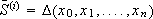is defined as,

where and .

Let us suppose, for simplicity, that the domain D is in . If a boundary configuration is defined such that the domain is partitioned in proper simplices, and a value of the function is associated to each intersection S ⁽ⁱ⁾ (or vertex), as shown in Fig. 2, it is possible to define a PWL function with the following characteristics,

• The function values assigned to each vertex define a unique (and local) linear affine function for each simplex.
• The local linear expressions define a PWL continuous function because they are continuous on the boundaries of the partition.

Figure 2: Simplex partition in ²

The extension of this idea to an m-dimensional domain leads us to define simplices of m + 1 vertices. Then, if one function value is associated to each vertex, it is possible to determine a unique linear affine (local) function for each simplex. In this way, a continuous PWL function is determined by the collection of all the local functions. From this procedure, it is clear that any arbitrary PWL function defined over the simplicial boundary configuration introduced is uniquely determined by its values on the vertices.

Next, without loss of generality, it is assumed that the dimension of the image set is one; because a PWL map from to is equivalent to m independent PWL maps from to with the same boundary configuration.

Definition 3: Consider a compact domain and a set of hyperplanes H. Then, PWL_H[D] is defined as the set of all the PWL continuous mappings taking values on the domain D partitioned with the boundary configuration H.

Julián (1999) proved that a set of HL CPWL functions which is a basis of PWL_H[D] was found as a function of m nesting absolute values (Julian et al., 1999). In addition, a set of generating functions for this base can be expressed in a vectorial form as

Theorem 1: The PWL functions of the set of functions are a basis for a linear vectorial space PWL_H[D]

For the proof of this theorem, see Julián (1999).

Then, any PWL function f Î PWL_H[D] can be univocally written as a linear combination of entries of as .

III. PWL FUNCTION APPROXIMATION

In this section, let us consider the approximation of a generic nonlinear function using a PWL realization. Specifically, the problem of uncertainty characterization for application in analysis and design of robust systems will be considered. To perform a robust approximation, Julián and Agamennoni (1999), assume that the measures to be approximated present uncertainties. In general, a function is called uncertain if it is characterized by a family of functions of the form

where f_N is a nominal function and D satisfies In addition, let us consider that a set F = {f₁, f₂, f₃, ..., f_s} of s measured values (members of ) over a set of points in the domain (V = {v₁, v₂, v₃, ..., v_s}) is available (i.e., f_i = f(v_i) with and ).

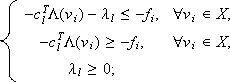
Julián (1999, 2000) proposes an algorithm to adjust a function f_p Î PWL_H[D] to measured points F using a Least Square criterion. In this case, we are looking for a complete set of uncertain functions. A natural way to perform this is to find an "upper" function, f_u Î PWL_H[D] and a "lower" function f_l Î PWL_H[D], satisfying

to characterize the uncertain function, in the sense that f can be represented as

f(v_i) = af_l(v_i) + (1 - a)f_u(v_i),

where 1 ³ a ³ 0. The "band" defined by these two functions should be as narrow as possible. This is equivalent to find the two functions, f_l and f_u, that solve the following optimization problems

Problem 1:

(1)

Problem 2:

(2)

Julián and Agamennoni (1999) show that these problems can be written as two Linear Programming problems. First, it will be considered that the upper and lower functions have PWL expressions ( and ).

Lemma 1: Let V, F, H and D be as described above. The Problems and can be stated as the linear programming problems

min l_l s.t.

(3)

2) min l_u s.t.

(4)

on the parameters c_u, c_l, l_u and l_l.

The computational experience has shown that the bounds of (1) and (2) could be conservative because single margins (l₁ and l_u) are used for the entire domain D. It is possible to define a particular margin l for each simplex in the partition of D. In this way, a less conservative margin is obtained as it will be shown in the application example.

IV. WIENER MODEL IDENTIFICATION

Various Wiener model identification approaches can be found in the literature.

• The N-L approach: First the output static nonlinearity is determined using steady state data, then the dynamic linear block is identified, where the intermediate signal v is generated from the output signal using inverse non-linearity mapping.
• The L-N approach: First the linear block is identified using a least squares estimation; after that the intermediate signal v is generated from the input signal and the static nonlinearity is estimated.
• The simultaneous approach: Parameters of the linear block and the static nonlinearity are estimated at the same time.

The second approach is used in this paper because is straightforward and it allows an accurate description of the static nonlinearity. In a first step the linear block is identified using a least squares estimation of a ARX model. The data to perform this identification is generated applying to the process a Pseudo Random Binary Signal. This ARX model may be easily transformed in a state space model.

In a second step, the static nonlinear block and the uncertainty bounds are identified. The identification data is obtained from experimentation by introducing several steps inputs to get information of the gain in the operation domain. Using this information, the PWL Toolbox proposed by Julián (1999, 2000), based on the Least Squares method, is used.

A combination of dynamic as well as stationary data were used in the evaluation of the uncertainty bounds. To compute these bounds the optimization problems (3) and (4) are solved.

A. Inverse Model

In order to implement the NMPC scheme, described in next section, a good representation of the inverse of the nonlinearity is needed. First, it is important to notice that the domain and the image of all the PWL functions (f, f_u and f_l) share the dimension (i.e., they are biyective functions). A large set of processes present this property in the neighborhood of the operative point. Then, it is possible to define the inverse function as f^-1 ( or ), such that v = f^-1(f(v)) ( or ). These functions are also unique and PWL. In order to obtain a description of such inverses, a set of input-output data is obtained for the vertexes of the partition and a PWL function from y to v is approximated.

V. WMPC UNDER UNCERTAINTY

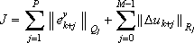
The control problem to be solved is to compute a sequence of inputs u_k, {k = 1, ..., M}} that will minimize the following dynamic objective:

subject to a model equations and to some inequality constraints

(5)

where P is the predictive horizon, M is the control horizon, is the deviation of the output from the desired set point r, Du_k+j = u_k+j - u_k+j-1 and the relative importance of the objective function contributions is controlled by setting the time dependent weight matrices Q_j and R_j. Beyond the control horizon the control signal is assumed to be constant (i.e. Du_k+j = 0, j = M, ..., P). Disturbances are typically handled by assuming that a step disturbance has entered the output and that it will remain constant for all future time (d_k = d_k+j, j = 1, ..., M). To accomplish this, a bias term that compares the current predicted output y_k to the current measured is computed:

Once u_k is computed, following the receding horizon principle, only the first element of the optimal control sequence is used as the current control value. Then, the horizon shifts one step forward in time and the whole procedure is repeated.

The state vector at the present time is assumed to be known and the future behavior of the variables is written in a matricial form as,

Then, the predicted output for the linear model is

where

and

Then the predicted output for the complete model is

Let us now define some points related to the MPC structure:

1. Since the PWL function f was assumed to be invertible, it is possible to write the desired signal referred to the output of the linear model as a transformation of the set point r(k) as,
   r^*(k) = f^-1(r(k))
2. If y_u and y_l are the upper and lower bounds for the outputs variables (y(k)), then we can translate these magnitudes to the linear model writing
   v_u(k) = f ^-1(y_u(k))
   v_l(k) = f ^-1(y_l(k))
3. In this case the disturbance is computed:
   
   where is the current predicted output for the linear model and y^m(k) is the current measure output for the process. It is straightforward to show that introducing this bias in the error expression, the model errors offset in steady state is removed.

Finally, the nominal WMPC can be posed as a quadratic optimization problem (QP),

(6)

s.t.

where the relative importance of the objective function contributions is controlled by setting the weight matrices Q and R. Note that minimization of (6) is a classical LMPC; then all properties about convergence to the global optimal solution and stability of the loop are guaranteed. Moreover, we can use the information of the uncertainty available from the nonlinear identification to guarantee no constraint violations along the process operation. To do this, we should transform the constraint bounds as

Note that the structure of the minimization problem does not change.

VI. CASE STUDY: NEUTRALIZATION REACTOR

A. Process Description

We shall consider a continuous stirred-tank reactor (CSTR) with a constant volume V, where an acid solution with a time varying volumetric flow q_A(t) ¹ 0 of a fixed composition x_1,i (acid) is neutralized with an alkaline solution with volumetric flow q_B(t) of known composition made up of base (x_2,i), and a buffer agent (x_3,i). The differential equations that describe the dynamic behavior of this process are given as (Galán, 2000),

	(7)
	(8)
	(9)
	(10)

Equation (10) can also be expressed in the polynomial form as,

where x = 10^-y, q = V/q_A and u = q_B /q_A. Equations (7 to 9) are mass balances of Equivalent Chemical Species, referred to in the literature as Chemical Invariants and Equation (10) is the well known pH equation (Galán, 2000). The nominal parameter values appear in Table 1.

Table 1: Model parameters.

A.1. Data preprocessing

It is important to study the data distribution in order to estimate the generalization properties of the resulting model (Abrahantes and Agamennoni, 2001). The simplicial partition used in the PWL formulation allows an easy determination of the number of points in each simplex. This information may be used to study the distribution of the data in the PWL input domain. A uniform distribution of data is generally associated with good generalization properties of a model. Figure 3 shows the number of data points in each simplex. From this picture it is clear that the steady-state data is satisfactory.

Figure 3: Number of samples in each simplex.

B. Process Identification

B.1. Linear identification

To perform the dynamic identification, a Pseudo Random Binary Signal was applied to the process on the nominal operating point (q_B = 0.5l/ min). The switching time was 1 minute with an amplitude of +/- 30%. The data was sampled every 0.1 minutes, during 200 minutes. Then, using 1500 samples of this data, an ARX model was adjusted using a least squares algorithm. The following model is obtained:

B.2. PWL identification

Having that linear model, several steady-state experiments were carried out and a PWL model was obtained using the PWL Toolbox (Julián, 2000). Using the same tool, a PWL description of the inverse of the nonlinear block was obtained. These static models are shown in Fig. 4. This plot includes the plot of expression and the PWL approximation. It is clear that the approximation using 50 sectors is almost perfect. The performance of the complete model can be appreciated in Fig. 5, where the comparison of the process and model outputs are shown for the set of data not used in the dynamic identification.

B.3. Uncertainty characterization

To evaluate the uncertainty, the bounds described in Eqns. (3) and (4) were computed using the combination of steady state and dynamic data. The addition of the dynamic data improves the information available in the central part of the operative region. The results are included in Fig. 6. In this case, an unique parameter l_l (and l_u) is used. To reduce the conservatism, the change proposed in order to consider different values of l_l (and l_u) for each simplice was implemented. The resulting bounds are shown in Fig. 7. It is clear that the conservatism was reduced. The inverses of these PWL are shown in Fig. 8.

C. Nonlinear Model Predictive Control

The control formulation described in Eqn. (6) was implemented for the neutralization reactor. The weighting matrices and the bounds on the variables are shown on Table 2. The simulation results are depicted in Figs. 9, 10 and 11 for the Robust WMPC, the nominal WMPC and linear MPC, respectively. It is clear, that the robust WMPC follows the set point better than the other controllers. Figure 12 shows the manipulated actions for the robust case.

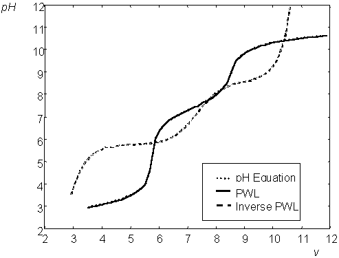
Figure 4: Nominal PWL approximation and its inverse.

Figure 5: Process and Model outputs.

Table 2: NMPC Parameters

Figure 6: Bounds for Steady State and Dynamic Data.

Figure 7: Bounds for Steady State and Dynamic Data computed with the modified problem.

Figure 8: Inverse of bounds.

VII. CONCLUSIONS

In this paper some considerations related with robust identification of Wiener models with PWL gain are analyzed. A Nonlinear Model Predictive Control based on such models is presented. By assuming invertibility in the nonlinear static function, a set point change allows to transform the nonlinear MPC into a linear MPC. It was also clearly showed that the modeling strategy used allows a simple gain uncertainty description, from which a robustness result related with no constrain violation in the feedback loop are naturally introduced. The performance of the controller is tested by simulation of a reactor of neutralization.

Figure 9: Process output for robust WMPC.

Figure 10: Process output for nominal WMPC.

Figure 11: Process output for linear WMPC.

Figure 12: Manipulated variable for robust WMPC.

REFERENCES
1. Abrahantes, M. and O. Agamennoni, "Approximate models for Nonlinear Dynamical Systems and its Generalization Properties", Mathematical and Computer Modelling, 33, 8-9, (2001).         [ Links ]
2. Bequette, B.W., "Nonlinear Control of Chemical Processes: A Review", Ind. Eng. Chem. Res., 30, 1391-1413, (1991).         [ Links ]
3. Castro, L., P. Julián, O. Agamennoni and A. Desages, "Wiener Modelling Using Canonical Piecewise Linear Functions", Latin American Applied Research, 29(3/4) , 265-272, (1999).         [ Links ]
4. Chua, L.O., "Efficient computer algorithms for piecewise-linear analysis of resistive nonlinear networks", IEEE Trans. Circuits Theory, CT-18, 73-85, (1971).         [ Links ]
5. Galán, O., "Robust Multi-Linear Model-Based Control for Nonlinear Plants", PhD Thesis, The University of Sydney, Australia, (2000).         [ Links ]
6. Galán, O., J.A. Romagnoli, and A. Palazoglu, "Robust H-infinity Control of Nonlinear Plants Based on Multi-linear Models - An application to a Bench pH Neutralization Reactor", Chem. Eng. Sci., 55, 4435-4450, (2000).         [ Links ]
7. Gerksic, S., D. Juricíc, S. Strmcnik and D. Matko, "Wiener Model based Nonlinear Predictive Control", Int. J. of Systems Science, 31, 189-202, (2000).         [ Links ]
8. Henson, M.A., "Nonlinear Model Predictive Control: current status and future directions", Computers and Chemical Engineering, 23, 187-202, (1998).         [ Links ]
9. Julián, P., High Level Canonical Piecewise Linear Representation: Theory and Applications, PhD Thesis, Universidad Nacional del Sur, Bahía Blanca, Argentina, (1999).         [ Links ]
10. Julián, P., A. Desages and O. Agamennoni, "High Level Canonical Piecewise Linear Representation Using a Simplicial Partition", IEEE Trans. Circuits Syst. I, 46, 463-480, (1999).         [ Links ]
11. Julián, P. and O. Agamennoni, "Tools for the PWL Approximation of Continuous Functions", Modern applied mathematics techniques in circuits, systems and control. Nikos E. Mastorakis (editor), Military Inst. of Univ. Educ. Hellenic Naval Acad., World Sci. and Engng. Soc. Press, 199-204,(1999).         [ Links ]
12. Julián, P., "A Toolbox for the Piecewise Linear Approximation of Multidimensional Functions", http://www.pedrojulian.com, (2000).         [ Links ]
13. Norquay, S.J., A. Palazoglu and J.A. Romagnoli, "Model Predictive Control Based on Wiener Models", Chem. Eng. Sci., 53, 75-84, (1998).         [ Links ]
14. Norquay, S.J., A. Palazoglu and J.A. Romagnoli, "Application of Wiener Model Predictive Control (WMPC) to pH Neutralization Experiment", IEEE Trans. Control System Technology, 7, 437-445, (1999a).         [ Links ]
15. Norquay, S.J., A. Palazoglu and J.A. Romagnoli, "Application of Wiener Model Predictive Control to an Industrial C2-Splitter", J. of Process Control, 9, 461-473, (1999b).         [ Links ]
16. Qin, S.J. and T.A. Badgwell, "An Overview of Industrial Model Predictive Control Technology", Fifth International Conference on Chemical Process Control, Eds.Kantor, Garcia and Carnahan, AIChe Symposium Series, 93, 232-257 (1997).         [ Links ]
17. Westwick, D., and M. Verhaegen, "Identifying MIMO Wiener systems using subspace model identification methods", Signal Processing, 52, 135-258, (1996).         [ Links ]