Frequency domain approach to Hopf bifurcation for van der Pol equation with distributed delay

Shaowen Li ^{1, 2} , Xiaofeng Liao ^{1, 3} and Shaorong Li ¹

¹ College of Electronic Engineering, University of Electronic Science and Technology of China, Chengdu, China;
² Department of Mathematics, Southwest University of Finance and Economics, Chengdu 610074, P. R. China;
lisw@swufe.edu.cn
³ Department of Computer Sciences and Engineering, Chongqing University, Chongqing 400044, P. R. China.
xfliao@cqu.edu.cn

Abstract ¾ The van der Pol equation with a distributed time delay and a strong kernel is analyzed. Its linear stability is investigated by employing the generalized Nyquist stability and Routh-Hurwitz criteria. Moreover, local asymptotic stability conditions are also derived in the case of the strong kernel. By using the mean time delay as a bifurcation parameter, the model is found to undergo a sequence of Hopf bifurcations. The direction and the stability criteria of the bifurcating periodic solutions are obtained by the graphical Hopf bifurcation theory. Some numerical simulation examples for justifying the theoretical analysis are also given.

Keywords ¾ Van der Pol Equation. Distributed Delay. Hopf Bifurcation. Periodic Solutions. A Polycyclic Configuration.

I. Introduction
The classical van der Pol equation, which describes the oscillations in a vacuum tube circuit, is the second-order nonlinear damped system governed by

, (1)

where f(x) = ax + bx³.
System (1) is considered as one of the most intensely studied systems in nonlinear dynamics (Guckenheimer and Holmes, 1983) and has served as a basic model of self-excited oscillations in physics, electronics, biology, neurology and other disciplines. Many efforts have been made to find its approximate solutions (Buonomo, 1998; Frey and Douglas, 1998; Guckenheimer and Holmes, 1983; Venkatasubramanian and Vaithianathan, 1994) or to construct simple maps that qualitatively describe the important features of its dynamics. Hence, if a > 0 and b > 0 in f(x), the origin is globally asymptotically stable and so there is no periodic solution for system (1). However, if a < 0 and b > 0, a unique stable periodic solution does exist.
It would be very useful if we have some knowledge about the existence of periodic solutions for delay nonlinear differential equations. As we know, in ordinary differential equations, one of the simple ways in which a non-constant periodic solution can arise is through Hopf bifurcation. This occurs when two eigenvalues cross the imaginary axis from left to right as a real parameter in the equation passes through a critical value (Gopalsamy, 1992; Hale and Verduyn, 1993; Hassard et al., 1981; Iooss and Joseph, 1989; Kung, 1992; MacDonald, 1989). In a study of classical van der Pol oscillators, it has been shown that oscillations occur when a stable equilibrium undergoes the singularity induced bifurcation in the slow differential-algebraic model, which, in turn, corresponds to the occurrence of supercritical Hopf bifurcations in the singularly perturbed models (Venkatasubramanian and Vaithianathan, 1994). Frey and Douglas (1998) proposed a class of relaxation algorithms for finding the periodic steady-state solution of a van der Pol oscillation. Buonomo (1998) gave the periodic solution of the van der Pol equation in the form of a series converging for all values of the damping parameter. Recently, discrete time delay was introduced into system (1) and the following pair of delay differential equations obtained (Murakaimi, 1999).

. (2)

No periodic solution is expected for a > 0 and b > 0 for the case where t > 0. Contrary to this, numerical simulations indicate that, under this condition, Eq. (2) could have a stable periodic solution. Murakaimi (1999) analyzed the existence of a periodic solution in detail by using the center manifold approach. However, the stability of the periodic solution is not investigated.
It is well known that dynamical systems with distributed delay are more general than those with discrete delay. This is because the distributed delay becomes a discrete one when the delay kernel is a delta function at a certain time. Dynamical systems with distributed delay have been found in population dynamics and neural networks (Atay, 1998; Bélair and Dufour, 1996; Bélair et al., 1996; De Vries and Principe, 1992; Gilsinn, 2002; Gopalsamy, 1992; Gopalsamy and Leung, 1997; Hopfield, 1984; Kung 1992; Liao et al., 1999; Marcus and Westervelt, 1989; Rasmussen et al., 2003; Stepan, 1986). In both biological and artificial neural networks, time delays arise as a result of the finite processing time of information. More specifically, in the electronic implementation of analog neural networks, time delays occur in the communication between and the response of neurons owing to the finite switching time of amplifiers. Usually, fixed time delays in models of delayed feedback systems can sufficiently approximate simple circuits having only a small number of cells. However, due to the spatial nature of the dynamical system resulting from the parallel pathways of a variety of system states, it is desirable to model them using distributed delays.
Liao et al. (2001) introduced the distributed delay with weak kernel into the van der Pol equation for studying the existence of Hopf bifurcation and the stability of the bifurcating periodic solutions. Their study found that both of them depend on the parameters a, b and the delay. In this paper, distributed delay with strong kernel will be introduced into the van der Pol equation. The existence of Hopf bifurcation, as well as the stability and the direction of the bifurcating periodic solutions, are obtained by applying the graphical Hopf bifurcation theory (Moiola and Chen, 1996). It is worth noting that information other than on the stability, can be deduced by other methods such as the center manifold theorem, the Fredholm alternative, implicit function theorem, the method of averaging, or the Poincaré-Lindstedt algorithm (Marsden and McCracken, 1976). However, the approach based on the graphical Hopf bifurcation theory has some advantages over the classical time-domain methods. A typical one is its pictorial characteristic that utilizes advanced computer graphical capabilities thereby bypassing quite a lot of profound and difficult mathematical analysis. A polycyclic configuration in the phase graph will be found by the graphical Hopf bifurcation theory (Moiola and Chen, 1996). This is especially prominent for the case of the following Eq. (3) with a strong kernel, since it is very difficult to determine the stability of the bifurcating periodic solutions by applying the time-domain approach in this case. Throughout this paper we substantially follow the method and the results (Moiola and Chen, 1996) and only give brief comments on the theory. The interested reader may refer to that book for a complete analysis.
The organization of this paper is as follows. In Section 2, the van der Pol equation with distributed delay is introduced. Its local stability is also discussed in detail. Some sufficient conditions for the existence of Hopf bifurcation are derived. The direction of Hopf bifurcation and the stability of the bifurcating periodic solutions are analyzed by using the graphical Hopf bifurcation theory (Moiola and Chen, 1996) in Section 3. In Section 4, numerical simulations aimed at justifying the theoretical analysis are reported. In Section 5, conclusions are drawn and further research directions are also given.

II. Local Stability and Hopf Bifurcation
In this section, we consider the following van der Pol equation with distributed delay

, (3)

where f(x) = ax + bx³.
The weight function k(s) is a non-negative bounded function defined on [0,+ ¥] that reflects the influence of the past states on the current dynamics. It is assumed that in this model the presence of the distributed delay does not affect the equilibrium values. Therefore, we normalize the kernel as follows:

.(4)

Usually, we employ the following form

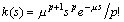
for the kernel. The kernel is called the 'weak' when p = 0, and 'strong' when p = 1, respectively. In this paper, a strong kernel is considered only, i.e.,

, (5)

where m reflect the mean delay of the strong kernel. For convenience, we set

. (6)

Then Eq. (3) is equivalent to the following model:

. (7)

Suppose that

f Î C⁴(R), and uf(u) > 0 for u ¹ 0. (8)

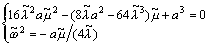
We will first consider a general function f that satisfies Eq. (8). Then, we can easily apply the conclusion to the case f(x) = ax + bx³. It is clear that the origin (0,0) is a stationary point of Eq. (3) or Eq. (7). As a result, Eq. (7) can be written as

. (9)

By , we have:

. (10)

Using Eq. (10) and taking the derivative with respective to t on both sides of Eq. (9), we obtain:

. (11)

Then, we take the derivative again with respective to t on both sides of Eq. (11).

. (12)

Letting , and , we get a six-dimensional ODE system:

. (13)

We rewrite the nonlinear Eq. (13) in a matrix form:

, (14)

where ,

,

H(x) = (0 0 0 0 -m² f(x₁) 0)^T. (15)

Now, we use the mean delay m as the bifurcation parameter. Then by introducing a "state-feedback control" u = g(y ; m), we obtain a linear system with a nonlinear feedback as follows:

, (16)

B = (0 0 0 0 -m² 0)^T,
C = (-1 0 0 0 0 0), u = g(y ; m) = f(y). (17)

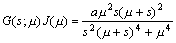
Next, taking a Laplace transform on Eq. (16), we obtain the standard transfer matrix of the linear part of the system:

. (18)

Now, if we linearize the feedback system about the equilibrium y = 0, the Jacobian is given by

. (19)

where a = f ' (0). So we have:

. (20)

Set

. (21)

Next, an application of the generalized Nyquist stability criterion, with s = iw, provides the following results:
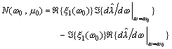
Lemma 1 (Moiola and Chen, 1996). If an eigenvalue of the corresponding Jacobian of the nonlinear system, in the time domain, assumes a purely imaginary value iw₀ at a particular m = m₀, then the corresponding eigenvalue of the constant matrix in the frequency domain must assume the value -1 + i0 at m = m₀.
Let be the eigenvalue of that satisfies . Then

. (22)

So the Eq. (22) becomes

. (23)

By separating this equation into real and imaginary parts, we obtain

, (24)
. (25)

So we have:

, (26)

or

. (27)

The roots of 4m² - 2am + 1 = 0 are

, (28)

and the roots of are

. (29)

So, we note

. (30)

Now, we examine the linearized equation of Eq. (13) at the origin. The characteristic equation of the linearized system is

. (31)

So, we have:

. (32)

Define

j1(m) = 4m,
	,

,

,

,

. (33)

A set of necessary and sufficient conditions for all the roots of Eq. (32) to have a negative real part is given by the well-known Routh-Hurwitz criteria in the following form:

j₁(m) = 4m, j₂(m) = 20m³ - am² > 0,
j₃(m) = (4m - a)(16m + a)m⁴ > 0,
,
,

. (34)

Noticing m_ £ a/4 if a > 0, we have j₃(m) < 0 if 0 < m < m_. From Eq. (34) it is found that all the roots of Eq. (32) have a negative real part if and only if:
a > 0 and m > m₊ . (35)
By the above analysis, we immediately have the following result.
Theorem 1. Local Stability and Existence of Hopf bifurcation
If a > 0 and m > m₊, then Eq. (3) is locally asymptotically stable at (0, 0). If a £ 0 or 0 < m < m₊, then Eq. (3) is unstable at (0, 0). m₊ is defined as Eq. (30).
1. If a > 2, then is the Hopf bifurcation of Eq. (3).
2. If a = 2, then m = m₊ = 1/2 is a codimension two bifurcation of Eq. (3).
3. If 0 < a < 2, then is the Hopf bifurcation of Eq. (3).
4. If a £ 0, then the Hopf bifurcation of Eq. (3) doesn't exist.
Remark: When m pass though m_, the number of the positive real eigenvalues will be changed from 4 to 2. Then the stability of (0, 0) will not be changed.

III. Stability of bifurcating periodic solutions
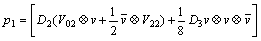
In order to study stability of bifurcating periodic solutions, we first define an auxiliary vector

, (36)

where is the fixed value of the parameter m, w^T and v are the left and right eigenvectors of , respectively, associated with the value , and

, (37)

where is the frequency of the intersection between the locus and the negative real axis closet to the point (-1 + i0), Ä is the tensor product operator, and

, ,
,

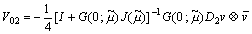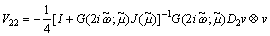. (38)

As and g(y ; m) = f(y), then we have

D₂ = f''(0), D₃ = f''(0), v = w = 1, (39)

and

V₀₂ = 0,

. (40)

Then

, (41)

and

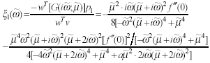. (42)

As is the eigenvalue of , we have

. (43)

We obtain

. (44)

Notice that is a real number. By separating Eq. (43) into real and imaginary parts:

, (45)
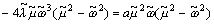. (46)

So, we obtain the following equation:

or

. (47)

Now, the following Hopf Bifurcation Theorem formulated in the frequency domain can be established:
Lemma 2. Suppose that the locus of the distinguished characteristic function intersects the negative real axis at that is closest to the point (-1 + i0) when the variable s sweeps on the classical Nyquist contour. Moreover, suppose that is nonzero and the half-line L₁ starting from (-1 + i0) in the direction defined by first intersects the locus of at , where . Finally, suppose that following conditions are satisfied:
(i) The eigenlocus has nonzero rate of change with respect to its parameterization at the criticality (w₀, m₀), i.e.,

, (48)

where .
(ii) The intersection is transversal, i.e.

. (49)

(iii) There are no other intersections between any of the characteristic loci and the line segment joining the point (-1 + i0) to , at least within a small neighborhood of radios d > 0.
Then, the system given by Eq. (9) has a periodic solution y(t) of frequency . Moreover, by applying a small perturbation around the intersection and using the generalized Nyquist stability criterion, the stability of the periodic solution y(t) can be determined.
According to Lemma 2, we can determine the direction of Hopf bifurcation and the stability of the bifurcating periodic solution by drawing the figure of the half-line L₁ and the locus .

1. If the half-line L₁ first intersects the locus of when , then the bifurcating periodic solution exists and the Hopf bifurcation is supercritical (subcritical).
2. If the total number of anticlockwise encirclements of the point , for a small enough e > 0, is equal to the number of poles of l(s)

that have positive real parts, then the limit cycle is stable, otherwise it is unstable.
We perturb the bifurcation parameter m slightly from m₀ to . If and , or and , then the half-line L₁ intersects the locus of .
By using m instead of in Eq. (47), and taking the derivative with respect to m on both sides of Eq. (47), and setting , and considering Theorem 1, we have:

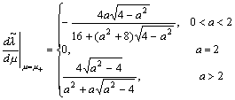. (50)

So, if 0 < a < 2 and if a > 2. We consider Eq. (43)
.
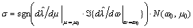
Now fixing m at , and taking the derivative with respect to w on both sides of Eq. (43), so we have:

. (51)

Setting , and considering Eqs. (26), (27) and (30), we obtain:

	, (52)
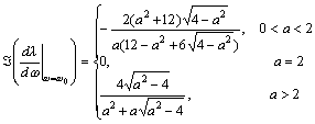	. (53)

Theorem 2. Set

. (54)

1. If s > 0, then the Hopf bifurcation m = m₀ of Eq. (3) is supercritical.

2. If s < 0, then the Hopf bifurcation m = m₀ of Eq. (3) is subcritical.
Now, we set f(u) = au + bu³, then f'(0) = a, f''(0) = 0, f''(0) = 6b. So in Eqs. (40), (41) and (44), we have:

V₀₂V₂₂ = 0, p₁ = f''(0)/8,

and

. (55)

Letting 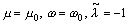, we can calculate

,

and

.

Considering is a real, i.e., 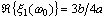, , and supposing a > 0 and a ¹ 2, we have:

.

According to Eqs. (44) and (45), if a > 2, and if 0 < a < 2. Therefore, if a > 2 and b < 0, or 0 < a < 2 and b > 0, sgn(s) < 0 at m = m₊; if a > 2 and b > 0, or 0 < a < 2 and b < 0, sgn(s) > 0 at m = m₊. Then
Corollary 1. Let f(u) = au + bu³, a > 2 and a ¹ 2.
1. If a > 2 and b < 0, or 0 < a < 2 and b > 0, the Hopf bifurcation at m = m₊ of Eq. (3) is subcritical;
2. If a > 2 and b > 0, or 0 < a < 2 and b < 0, the Hopf bifurcation at m = m₊ of Eq.(3) is supercritical.
Then, one draws the half-line starting from (-1 + i0) and the locus , and obtains the total number k of anticlockwise encirclements of the point for a small enough e > 0.
According to Eq. (21), one has

. (56)

Hence, the roots of s²(s + m)⁴ + m⁴ = 0 are the poles of l(s). According to the Routh -Hurwitz criteria, the number of poles of l(s) that have positive real parts is two.
Corollary 2. Let k be the total number of anticlockwise encirclements of the point for a small enough e > 0, where is the intersection of the half-line L₁ and the locus . Then:
1. if k = 2, the bifurcating periodic solutions of Eq. (3) is stable;
2. if k ¹ 2, the bifurcating periodic solutions of Eq. (3) is unstable.

IV. Numerical Examples
In this section, some numerical examples of Eq. (3), with Eq. (5) at different values of a and b, are discussed. By Corollary 1, b determines the direction of a Hopf bifurcation. If a > 2 and b < 0, or 0 < a < 2 and b > 0, the Hopf bifurcation m₊ is subcritical; if b < 0 and b > 0, or 0 < a < 2 and b < 0, the Hopf bifurcation m₊ is supercritical. The half-line L₁ and the locus are shown in the corresponding frequency graphs. If they intersect, a limit cycle exists, or else, no limit cycle exists. By Corollary 2, the stability of the bifurcating periodic solutions is determined by the total number k of anticlockwise encirclements of the point for a small enough e > 0. Suppose that the half-line L₁ and the locus intersect. If k = 2, the bifurcating periodic solutions is stable; if (-1 + i0), the bifurcating periodic solutions is unstable.
In order to verify the theoretical analysis results derived above, the half-line L₁ and the locus are shown in the corresponding frequency graphs, and Eq. (3) is simulated with Eq. (5) in different cases. We can observe that a smaller stable and a greater unstable periodic solution, i.e., a polycyclic configuration exists in the following cases, similar to the one obtained by Genesio and Bagni, 2003. However, the strictly theoretical analysis must use the high-order harmonic balance approximations (Moiola and Chen, 1996). In this paper, the analysis about this problem will not be presented. The interested reader may refer to (Moiola and Chen, 1996).
(i) Let a = 1, b = 3. Then, m₊ = 3.4821 is a Hopf bifurcation point. As a = 1 < 2 and b = 3 > 0, then m₊ = 3.4821 is a subcritical Hopf bifurcation point.

Fig 1.1 a = 1, b = 3, m = 3.4. The half-line L₁ intersects the locus twice, and k = 2 at the first intersection, k = 0 at the second, so a smaller stable and a greater unstable periodic solution, i.e. a polycyclic configuration exist.

Fig 1.2 a = 1, b = 3, m = 3.6. The half-line L₁ intersects the locus once, and k = 0, so an unstable periodic solution exists.

Fig 2.1 a = 3, b = -2, m = 1.2. The half-line L₁ intersects the locus twice, and k = 2 at the first intersection, k = 0 at the second, so a smaller stable and a greater unstable periodic solution, i.e. a polycyclic configuration exist.

(ii) Let a = 3, b = -2. Then, m₊ = 1.3090 is a Hopf bifurcation point. As a = 3 > 2 and b = -2 < 0, then m₊ = 1.3090 is a subcritical Hopf bifurcation point.

Fig 2.2 a = 3, b = -2, m = 1.4. The half-line L₁ intersect the locus once, and k = 0, so an unstable periodic solution exists.

V. Conclusions
The van der Pol equation with delays provides rich dynamical behavior. From the viewpoint of nonlinear dynamical systems, their analyses are useful in solving problems of both theoretical and practical importance.
By using the average time delay as a bifurcation parameter, we have shown that a Hopf bifurcation occurs when this parameter passes through a critical value, i.e., a family of periodic orbits bifurcates from the origin. The stability and direction of the bifurcating periodic orbits have also been analyzed by drawing the amplitude locus L₁ and the locus, , in a neighborhood of the Hopf bifurcation point. Parameter s or b was used to determine the direction of the Hopf bifurcation: if s > 0, the Hopf bifurcation is supercritical; if s < 0, the Hopf bifurcation is subcritical; but if s = 0 (i.e. parameter a = 2, m = 0.5) one cannot determine the direction of the bifurcating periodic orbits by only using L₁ and , in fact, m = 0.5 for a = 2 is a codimension two bifurcation. The analysis of codimension two bifurcation will be presented in another paper.

Acknowledgement
The authors would like to thank two reviewers for their constructive and valuable comments and suggestions. The work described in this paper was supported by a grant from the National Natural Science Foundation of China (No. 60271019), the Doctorate Foundation Grants from the National Education Committee of China (No. 20020611007), and the Scientific Research Fund of Southwestern University of Finance and Economics (No. 04X16).

References
1. Atay, F. M., "Van der Pol's oscillator under delayed feedback", Journal of Sound and Vibration, 218, 333-339 (1998).         [ Links ]
2. Bélair, J. and S. Dufour, "Stability in a three-dimensional system of delay-differential equation", Canadian Applied Mathematics Quarterly, 4, 135-156 (1996).         [ Links ]
3. Bélair, J., S. Campbell, and P. van den Driessche, "Frustration, stability and delay-induced oscillations in a neural network model", SIAM Journal Applied Mathematics, 56, 245-255 (1996).         [ Links ]
4. Buonomo, A., "The periodic solution of van der Pol's equation", SIAM Journal on Applied Mathematics, 59, 156-171 (1998).         [ Links ]
5. De Vries, B. and J. C. Principe, "The gamma model - A new neural model for temporal processing", Neural Networks, 5, 565-576 (1992).         [ Links ]
6. Frey, M. and R. Douglas, "A class of relaxation algorithms for finding the periodic steady-state solution", IEEE Transactions on Circuits and Systems, 45, 659-663 (1998).         [ Links ]
7. Genesio R. and G. Bagni, "A view on limit cycle bifurcations in relay feedback system," IEEE Transactions on Circuits and Systems, 50, 1134-1140, (2003).         [ Links ]
8. Gilsinn D. E., "Estimating critical Hopf bifurcation parameters for a second-order delay differential equation with application to machine tool chatter", Nonlinear Dynamics, 30, 103-154 (2002).         [ Links ]
9. Gopalsamy, K., Stability and Oscillation in Delay Differential Equations of Population Dynamics, Kluwer Academic Publishers, Boston, MA (1992).         [ Links ]
10. Gopalsamy, K. and I. Leung, "Convergence under dynamical thresholds with delays", IEEE Transactions on Neural Networks, 8, 341-348 (1997).         [ Links ]
11. Guckenheimer J. and P. J. Holmes, Nonlinear Oscillations, Dynamical System, and Bifurcations of Vector Fields, Springer-Verlag, Berlin (1983).         [ Links ]
12. Hale, J. and S. Verduyn Lunel, Introduction to Functional Differential Equations, Springer-Verlag, New York (1993).         [ Links ]
13. Hassard, B. D., N. D. Kazarinoff, and Y. H. Wan, Theory and Applications of Hopf Bifurcation, Cambridge University Press, Cambridge (1981).         [ Links ]
14. Hopfield, J. J., "Neurons with graded response have collective computational properties like those of two state neurons", Proceedings of National Academic Sciences, USA, 81, 3088-3092 (1984).         [ Links ]
15. Iooss, G. and D. D. Joseph, Elementary Stability and Bifurcation Theory, 2nd edition, Springer-Verlag, New York (1989).         [ Links ]
16. Kung, Y., Delay Differential Equations with Applications in Population Dynamics, Academic Press, New York (1992).         [ Links ]
17. Liao X. F., K. W. Wong and Z. F. Wu, "Hopf Bifurcation and Stability of Periodic Solutions for van der Pol Equation with Distributed Delay", Nonlinear Dynamics, 26, 23-44 (2001).         [ Links ]
18. Liao X. F., Z. F. Wu, and J. B. Yu, "Stability switches and bifurcation analysis of a neural network with continuously delay", IEEE Transactions on Systems, Man & Cybernetics - Part A, 29, 692-696 (1999).         [ Links ]
19. MacDonald, N., Biological Delay Systems: Linear Stability Theory, Cambridge University Press, Cambridge (1989).         [ Links ]
20. Marcus, C. M. and R. M. Westervelt, "Stability of analog neural network with delay", Physical Review A, 39, 1989, 347-359 (1989).         [ Links ]
21. Marsden, J. E. and M. McCracken, The Hopf Bifurcation and Its Applications, Applied Mathematics Sciences, Vol. 19, Springer-Verlag, Heidelberg (1976).         [ Links ]
22. Moiola J. L. and G. Chen, Hopf Bifurcation Analysis: A Frequency Domain Approach, World Scientific, Singapore (1996).         [ Links ]
23. Murakaimi, K., "Bifurcated periodic solutions for delayed van der Pol equation", Neural, Parallel & Scientific Computations, 7, 1-16 (1999).         [ Links ]
24. Rasmussen H., G. C. Wake and J. Donaldson, "Analysis of a class of distributed logistic differential equations", Mathematical and Computer Modelling, 38, 123-132 (2003).         [ Links ]
25. Stepan, G., "Great delay in a predator-prey model", Nonlinear Analysis, 10, 913-929 (1986).         [ Links ]
26. Venkatasubramanian, K. and P. Vaithianathan, "Singularity induced bifurcation and the van der Pol oscillator", IEEE Transactions on Circuits and Systems, 41, 765-769 (1994).         [ Links ]