


Servicios Personalizados
Revista

Articulo
 Inglés (pdf)
 Articulo en XML
 Referencias del artículo
 Enviar articulo por email
Indicadores
-
 Citado por SciELO
Links relacionados
-
 Similares en
SciELO
Similares en
SciELO
Compartir

 Permalink
Latin American applied research
versión impresa ISSN 0327-0793
Lat. Am. appl. res. v.36 n.2 Bahía Blanca abr./jun. 2006
On-line costate integration for nonlinear control
V. Constanza1 and C. E. Neuman2
1 Instituto de Desarrollo Tecnologico para la Industria Quimica (INTEC),UNL-CONICET,
Güemes 3450, 3000 Santa Fe, Argentina. E-mail: tsinoli@ceride.gov.ar
2 Mathematics Department, Fac. Ing. Quimica, Universidad Nacional del Litoral,
Santiago del Estero 2829, 3000 Santa Fe, Argentina. E-mail: cneuman@fiqus.unl.edu.ar
Abstract — The optimal feedback control of nonlinear chemical processes, specially for regulation and set-point changing, is attacked in this paper. A novel procedure based on the Hamiltonian equations associated to a bilinear approximation of the dynamics and a quadratic cost is presented. The usual boundary-value situation for the coupled state-costate system is transformed into an initial-value problem through the solution of a generalized algebraic Riccati equation. This allows to integrate the Hamiltonian equations on-line, and to construct the feedback law by using the costate solution trajectory. Results are shown applied to a classical nonlinear chemical reactor model, and compared against standard MPC and previous versions of bilinear-quadratic strategies based on power series expansions.
Keywords — Process Control. Nonlinear Dynamics. Optimization. Hamiltonian Systems.
I. INTRODUCTION
A diversity of control techniques still compete on applicability and efficiency for general nonlinear processes. Since nonlinearities and main qualitative features of industrial processes are often detected without having a complete mathematical description of their dynamics, some techniques are being developed to overcome the use of models in designing control laws. Partial Control is one of these novel decentralized strategies conceived for meeting multiple economic objectives by feedback control of a few 'dominant variables' (see Tyréus, 1999). The concept is appealing because, if successful, a few SISO control loops replace the conventional process model for control purposes. Individual loops are in principle simpler to treat, instrument, and tune than multidimensional interconnected situations.
The steady-states' phase-plots for nonlinear dynamics adopt different patterns, sometimes leading to bifurcations, limit cycles, or strange attractors in high dimensions (Strogatz, 1994; Costanza, 2005a). These patterns may change, even structurally, when parameters of the dynamics vary (equilibrium control values may be regarded as parameters, specially when each manipulated variable is proportional to some physical variable like temperature or flow rate (Aris, 1999). Consequently, changing operation from one steady-state to another may imply working near bifurcation points, where model information is essential.
Disjoint from heuristic methods there exist a range of model-based approaches, Model Predictive Control (MPC) becoming the most notorious. Still, for nonlinear systems MPC is only recommended in very special situations (Figueroa, 2001; Norquay et al., 1998) given the computational complexity of the calculations involved. Most successful industrial applications of MPC reported so far are in refining and petrochemical plants, where (continuous) processes are run near optimal steady-states and model linearizations are reliable approximations. Only one of the available commercial software packages was cautiously suggested for truly nonlinear or batch processes in a recent survey (Qin and Badgwell, 1997).
Some numerical implementations of MPC discretize the whole event space  ×
×  from the beginning, which for nonlinear systems have predictable shortcomings (an event is a pair (x, t) of a state x ∈ and a time instant t ∈ , denoting the state space and the time span under consideration. Trajectory perturbations are increasingly important in the nonlinear case, specially near unstable steady-states. Since states are allowed to take only discrete positions in the calculations, being near unstable equilibria may not be noticed by the algorithms. Contrarily, feedback laws are determined from ODE's parameters that contain all stability information. Also, control values calculated from these laws depend on the exact (actual) values of state variables. To attain the same degree of accuracy with the MPC approach involves refining the discretization (so increasing the computing time, which makes troublesome to keep on-line work), and guaranteeing convergence of this refining (rarely taken into account). Minimizing computing time in nonlinear MPC is not a trivial problem, as reflected by the variety of unrelated techniques (Hammerstein, Wiener, and ARX polynomials, neural networks, piecewise linear models) used to attack the resulting Nonlinear Programming set-up numerically. Basically MPC (except for some theoretically oriented versions) requires exploring and/or calculating the cost of many trajectories at many time instants. Also, some review literature asserts that MPC does not guarantee success in general MIMO systems situations (Sriniwas and Arkun, 1997).
In this paper an optimal control technique based on universal approximations of general systems coupled with quadratic-type expressions of the economic objectives is proposed for nonlinear processes, specially applicable to multivariable situations that are not reducible to single loops. Some positive features of both partial control and MPC approaches are present in this proposal, while avoiding their main limitations and inconveniences. Feedback control laws instead of nonlinear programming are adopted, as in the first class of techniques; but model-based rather than empirical knowledge guides the calculations, in accordance with the second class. Bilinear approximations describe the dynamics. They have shown to be able to approximate fairly general nonlinear systems under bounded control situations and for a prescribed time period (Fliess, 1975; Sussmann, 1976), a feature that linear systems can not meet in general (see for instance Krener, 1975). Bilinear models were introduced long ago in the chemical engineering literature (Cebuhar and Costanza, 1984), and since then a number of improvements have been devised to treat different control problems on these systems, like regulation, tracking, and filtering. In particular, the optimal state estimate (in the least-squares sense) for bilinear systems is the solution to the Kalman-Bucy differential equation (with a slightly different time-dependent linear coefficient, see Costanza and Neuman (1995) for details). The Kalman-Bucy equation can be integrated on-line, along with the control strategy devised in this paper.
Observation problems may arise in practical applications, where the initial state needs to be recovered from output measurements. An approach to the design of on-line nonlinear observers to cope with those situations has been illustrated in a recent article (Costanza, 2005b; the references may help in extending the strategy to other processes).
Another advantage of this method, in the regulation context, is its robustness. It is known that the optimal bilinear-quadratic solution generates a closed loop with infinite gain margin (Glad, 1987).
Chemical reactors are a classical source of problems in the nonlinear control literature, and a number of other nonlinear chemical processes are receiving increasing attention (Costanza, 2005a; Henson and Se-borg, 1997; Bequette, 1991). As a case-application a well known nonlinear reactor model is revisited here (Sistu and Bequette, 1995). Equations correspond to the 'series/parallel Van de Vusse reaction', taking place in an isothermal CSTR. There are clearly two species concentrations in the example that need to be controlled, and just one variable (a flow rate) available for manipulation. No I/O pairing is possible since both states must be measured and optimized, so they are also output variables. The graph of equilibrium control values contains closed curves in phase space, situation described as 'system with input multiplicities' in the literature. Therefore, changes in set point not always involve changes in the final equilibrium value of the manipulated variable (a parameter that may have been previously optimized).
Adaptive strategies will not be discussed here for simplicity. The formula used in the numerical examples were advanced in Costanza and Neuman (1995). Set-point changes are eventually treated as tracking problems (following Costanza and Neuman (2000)) for comparison with the typical servo formulation.
In the following sections we describe the control strategy, the system to be controlled, some numerical results and comparisons with other methods applied to the controlled process, and conclusions.
II. THE CONTROL STRATEGY.
Nonlinear control processes under consideration will be those accurately modeled by equations of the form
 = f(x, u), (1)
where the function f is at least continuously differentiable and the admissible control strategies are at least piecewise continuous, bounded functions of time t, the implicit independent variable taking values in an interval of the real numbers. States x are assumed to evolve in some open set  of the n-dimensional Euclidean space, so = in what follows, and just for simplicity of notation (Isidori, 1989) the control values will be taken as scalars. Under these conditions nonlinear systems can be universally approximated by bilinear models of the form
= Ax + (B + Nx)u, x(0) = x0, (2)
where the initial state x0 ∈ ⊂  n, real matrices A, B, and N having the appropriate orders. An equilibrium of the original system is a pair (
 ,
,  ) that makes f(, ) = 0. When the system evolves near such an equilibrium a natural bilinearization would be
  . The underlying objective function will be the classical quadratic cost JT(x0, 0, u(·)) referred to the (x, u) trajectories generated by control functions u(·), starting (when t = 0) at the state x(0) = x0, acting during a time span of duration (with horizon) T ∈ (0, ∞], and evaluated from
 | (3) |
where Q and S are positive semi-definite matrices (S = 0 for T = ∞), and r is a positive scalar. For the regulator problem, (, ) should be regarded as the original equilibrium (a pair where is a steady-state and the corresponding constant control value), and from which disturbances should be abated. Usually, in regulation problems the variables are defined relative to this equilibrium, and then assuming (, ) = (0,0) ∈ is appropriate. For the servo (or set-point change) problem no relative values for states or controls will be used, since there are more than one equilibrium involved: (, ) is the pair consisting of the target set-point and its corresponding equilibrium control, which usually should be reached from the original equilibrium (x0,u0). It will become clear that in the nonlinear context the servo problem can not be reduced to a relative regulator problem around the target set-point.
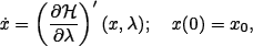
The Hamiltonian for the regulator problem can be written then
H(x, u, λ) = x'Qx + ru2 + λ'[Ax + (B + Nx)u]. (4)
Here the adjoint variable (or costate) λ is a column vector, associated in optimal control theory to the transpose of the (row) gradient ^ of the value function V defined by
 | (5) |
This Hamiltonian is regular (Kalman et al., 1969), and has the unique extremum
 | (6) |
which does not depend explicitly on t.
The Hamiltonian expression of this optimal control problem, (or its Hamiltonian equations, see for instance Sontag (1998)), takes the form of the following two-point boundary-value problem
 | (7) |
 | (8) |
where  . For regular Hamiltonians, to solve this boundary-value problem is equivalent to solve the Hamilton-Jacobi-Bellman (HJB) partial differential equation
 | (9) |
with the boundary condition
V(x,T) = x'Sx ∀x ∈ (10)
The regulator problem for an infinite horizon (T = ∞) has been solved (Cebuhar and Costanza, 1984) by proposing
 | (11) |
with P(x) an n × n symmetric matrix allowing a generalized power series expansion (see Costanza and Neuman, 2003; Cebuhar and Costanza, 1984; for details). Since there is no time-dependence of the value function, the HJB equation reads in this case
 | (12) |
W(x) being defined below. Equations for the series coefficients of P(x) were originally found from the conventional method of replacing the series expression into the HJB equation and collecting terms. The results of this approach have shown some practical inconveniences, since there exists no theoretical indication as to how many coefficients should be evaluated in each problem to obtain the desired accuracy for all state trajectories. The dimensions of the matrix coefficients Pi increase fast with the generalized power i, so it may become cumbersome to calculate, store, and use those coefficients to evaluate the feedback law in real time. In this paper a novel and simpler procedure is presented. By calling
 | (13) |
then, equation (12) is equivalent to
x'[Q + 2P(x)A - P(x)W(x)P(x)]x = 0, ∀x ∈ . (14)
Since P(x) was assumed symmetric, and equation (14) must be verified for all x in an open set that contains the origin, then it will be sufficient to ask
Q + P(x)A + A'P(x) - P(x)W(x)P(x) = 0 ∀x ∈ . (15)
Equation (15) is a Riccati equation for each x, of the same type as the Algebraic Riccati Equation (ARE) appearing in the classical linear-quadratic regulator problem, and therefore (see Sontag, 1998), under the restrictions imposed on the constant matrices, it is known that there exists a unique symmetric positive definite solution P(x) for each x.
This result allows then to write the optimal feedback law in the form
 | (16) |
Now, solving a Riccati equation for each x is not quite appropriate for on-line control in general, but the existence of P(x) is most useful. In fact, it is basic for the alternative method proposed below, which can be readily implemented in real time.
Actually, if Eq. (15) is solved just for x0, then the Hamiltonian equations associated to the optimal-control problem can be posed as an initial-value problem (see Eqs. (20) and (21)). Notice that for nonlinear systems, even in the infinite horizon case, the initial value for the costate λ is not known, so this formulation may be considered as an important indirect contribution of using bilinear models as approximations. It is also interesting to check, by making N = 0 in these equations, that the bilinear result is reduced to the well-known linear-quadratic steady-state solution, and P(x) = P, the solution to the standard ARE equation.
Summarizing, the new strategy for obtaining the optimal control of the bilinear-quadratic regulator problem would consist in: (i) solve equation (15) for P(x0), and then (ii) integrate the Hamiltonian equations online, which allows to evaluate the optimal control in feedback form by using the costate solution λ(·), i.e.
 | (17) |
For the servo problem, still in the infinite horizon case, the same type of strategy can be derived through the slightly different proposal
 | (18) |
where is the target set-point to which the initial state x0 (eventually the original set-point) should be driven. The extremum of the Hamiltonian is
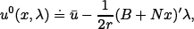 | (19) |
and the corresponding Hamiltonian equations in initial-value form can be written now:
 | (20) |
 | (21) |
where x(0) = x0, λ(0) = 2 (x0)(x0 - ) and
 A + N, also (x) is the unique symmetric positive definite solution to the Riccati equation
Q + (x) + '(x) - (x)W(x)(x) = 0. (22)
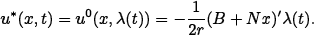
Formally, the optimal feedback law for the servo problem is then
 | (23) |
but in practice the on-line-appropriate form is
 | (24) |
where  (·) is the costate-part of the solution to equations (20-21).
A final observation: the Hamiltonian equations for the regulator problem may be recovered from equations (20-21) associated to the servo problem (simply put (, ) = (0,0)). But the converse is not true. If deviations from the target equilibrium, namely x - , u - , and their dynamics are replaced by x, u in the regulator equations, then the servo equations (20-21) are not obtained as written above unless the system is linear (N = 0). This shows that the regulator and servo problems are not equivalent in the nonlinear context, as announced.
III. A CLASSICAL NONLINEAR CHEMICAL PROCESS. THE FLOW STRUCTURE.
Consider an adiabatic CSTR in which the exothermic first-order irreversible Van de Vusse reaction is taking place (we follow the notation and order-reduction assumptions of Sistu and Bequette (1995)). The di-mensionless equations for the mass and heat balances are
 | (25) |
Typical values for the parameters are θ = 0,135, γ = 20,0, x1f = 1,0, β = 11,0, x2f = 0,0, and δ = 1,5, the variable x1 is the dimensionless extent of reaction and x2 is the dimensionless reactor temperature. The dimensionless feed flow rate q is the only variable that can be manipulated. Usually it is chosen to conduct operation around a fixed value q0 of the flowrate, and then an appropriate definition for the control variable would be u = q - q0. Since q0 is associated with flow rate, an operational problem arises when trying to change the (state) set-point without changing the final value of q (possibly dictated by the steady-state functioning of the rest of the plant) since the state trajectory must navigate through potentially adverse conditions as the structure of the flow changes.
IV. NUMERICAL SIMULATIONS
The two typical feedback control situations are explored for the reactor model of Section III: regulation control near an operational set-point, and optimal changes of set-point (typically from one steady-state of the system to another).
A. Regulation
In this case it will be assumed that a perturbation occurs when the reactor is conducted around the (generic) steady-state x = 0, and control is required to return the system to rest. The system is bilinearized near the steady-state, rendering the bilinear matrices: A, B, N. The optimization parameters are fixed at suitable values (Q = I associated to state deviations, and r = 0,33 to penalize the control effort). In practice these parameters should be consistent with the subjacent static optimization objectives decided at the designing level.
The goal in this regulation problem is to maintain the system near the steady-state = (0,932,0,501) with the minimum quadratic cost. As a first example the simulated initial states (post perturbation) are set at x0 = (1,4,0,9)
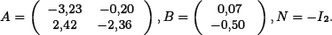
The bilinear approximation calculated through near equilibrium through partial derivatives of the original dynamics renders the matrices:
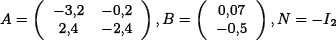
where I2 is the identity matrix in two dimensions.
The value of P( 0) at the original perturbation 0 = x - results
which is easily checked to be symmetric and positive-definite. Then, the initial value of the costate, needed to start integration of the Hamiltonian equations online is

The states and control trajectories resulting from the feedback law devised in Section 2, corresponding to the optimal bilinear-quadratic problem but applied to the original nonlinear dynamics, are shown in figures 1-2. These are also plotted and compared against the solution to the same problem obtained by using power series expansions, which results less accurate, probably due to truncation errors (coefficients only up to P2 were kept). Matrices A, b, N were automatically adapted using the software devised in Costanza and Neuman (1995), but the dimension of the bilinear model remains 2.
Figura 1: States deviations x -  vs. time trajectories for the regulation case. Steady-state = (0,932,0,501)' perturbed to (1,4,0,9)'. Equilibrium control q =
  = 3. The leftmost curves correspond to (x1 - 1) and the others to (x2 - 2).

Figura 2: Control deviation u - vs. time-trajectory for the regulation case. Steady-state: (0,932,0,501)' perturbed to (1,4,0,9)'. Equilibrium control = 3
The simulation also produced the costate trajectories (not depicted), which go to zero as desired; and the value of the Hamiltonian along the combined (x(·), ?(·)) trajectory, calculated from Eq. (12), which stays negligibly deviated from zero. This possibility of evaluating the Hamiltonian on-line (actually, of checking the whole HJB equation) may help to decide when to increase the dimension of the bilinear approximation.
The optimal control law works well in this case, despite the strongness of the simulated perturbation (around half the size of the desired values). This behavior may be inferred from the dynamics: the perturbed initial state lies in a region for which the flow trajectories do not change their qualitative pattern, and the values of q involved have little variation.
Another perturbation around the same , much smaller in size but differing in sign for the two states, is regulated with little effort (a small overshooting appears for one of the states), as shown in Figs. 3 and 4.

Figura 3: Evolution of regulated state variables. Steady-state: (0,0)' (relative), perturbed to (0,02,-0,02)'. Steady-state (absolute): = (0,932,0,501)'

Figura 4. Evolution of regulating control variable Steady-state. (0 0)' (relative), perturbed to (002-002)' Steady-state (absolute): = (0,932, 0,501)'
Perturbations being small, linear approximations may be intented. However (linear) Matlab MPC (see Fig. 5) results unable to send both states to zero simultaneously with just one manipulated variable, and also its cost is higher than the cost of the nonlinear strategy. The cumulative cost for this regulation process is about 0,075. Meanwhile, the correspondent MPC calculated cost (same units of measure) is 0,133. Therefore, when states are impaired with manipulated variables, a wholly nonlinear treatment results profitable besides than accurate.
Figura 5: States vs. time trajectories for the regulation case using MPC. Steady-state: (0,0)' (relative),perturbed to (0,02,-0,02)'. The uppermost curve corresponds to x1 and the lower one to x2.
B. Changes of set-point. The servo problem.
Operational flexibility may induce to change the set-point, which in principle has to be performed in an optimal fashion. Decisions of this kind have been reported in the classical Chemical Engineering literature, even conducting to unstable equilibria, usually obeying to 'new' economical restrictions.
The problem under consideration may be reformulated as one of tracking, with the reference trajectory xr(·) ≡ ∀t ∈ [0, T]. The tracking objective pursues the control u(·) that leads the initial state (eventually the original set-point) x0 to the target set-point in an optimal way. This problem has been treated in Costanza and Newman (2000) and the references herein, so only the relevant equations are recalled here.
The solution of the HJB equation was explained in Costanza and Newman (2003). Notice that the equations for the linear case correspond exactly to the ODEs for N = 0. In that case P1 plays the role of the gain coming from the solution to the standard Differential Riccati Equation (DRE). Then, increasing accuracy for nonlinear systems requires to keep more Pi's (which can be visualized as high order gains). Correspondingly, it will be necessary to solve 'backwards' an increasing number of simultaneous ODEs, and to keep all results in memory, since they will be finally used 'forwardly' when constructing the feedback law.
Change towards a stable set point
In Fig. 6 the process of change of set point between two stable set points of the system is illustrated. In this case the tracking goal is to lead the system to the state = (0,828,1,0) where the starting state is x0 = (0,932,0,5)
Figura 6: Relative states' trajectories (x - ) for the tracking case. Starting steady-state: x0 = (0,931877,0,5)' (old set point). New set point: = (0,828312, 1,0)', = 1,68812.
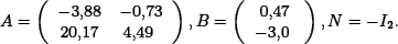
The initial bilinear approximation calculated for this case was calculated from partial derivatives of the nonlinear dynamics around x0:
The resulting trajectories of the Hamiltonian and the power series approaches to this case are shown in figure 6, where only minor differences appear. Optimal controls calculated by both methods are also very similar (not plotted).
A second example shows the change from an unstable set-point x0 = (0,528,3,0) towards the same (stable) steady-state used in the previous example.
The initial bilinearization resulted in this case
The evolution of the states is depicted in Fig. 7. Even when the initial set-point x0 in this example is an unstable steady-state of the system, the Hamiltonian strategy works equally well, as in the stable-to-stable case.

Figura 7: Relative states' trajectories (x - ) for the tracking case. Starting steady-state: x0 = (0,527964,3,0)' (old set point). New set point: = (0,828312,1,0)', = 1,68812.
Change towards a saddle (unstable) set point It is chosen here to illustrate the change from a stable to an unstable set-point, both steady-states corresponding to the same q-value = q*. The value of input flux may be bounded and/or fixed by production rate restrictions or for technical reasons, so this situation of keeping equal the original and final inputs may be desirable. It is also realizable for this particular system, because it presents the so called 'input multiplicity' property (Sistu and Bequette, 1995). Since q is the manipulated variable, a nontrivial optimal control has to move above and/or below q*.
In figures 8-9 this process of changing set-points from a stable x0 = (0,178, 6,031)' towards the unstable steady-state = (0,498, 3,682)' is illustrated.

Figura 8: Relative state variables (x - ) evolution for changing set points from steady-state: x0 = (0,178,6,031)' (old set point) to = (0,498,3,682)' (new set point), = q* = 3.
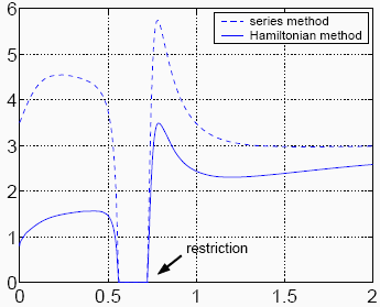
Figura 9: Control variable evolution for changing set points from steady-state: x0 = (0,178, 6,031)' (old set point) to = (0,498, 3,682)' (new set point), = q* = 3.
The bilinear approximation calculated for this case results

The main feature to remark from this example is the robustness of the optimal control strategy. Since the system has to go through adverse flow conditions to reach an unstable equilibrium, the evolutions of state and control variables are not monotonically smooth. They grow and decrease around the final desired values, reflecting the directions of the flow in the different regions of phase space. In a given moment (see figure 9) a restriction is applied to the control u = q, since it can not naturally assume negative values, but this instantaneous absence of control action has no adverse effect. This is an important consequence of working with optimal feedback control laws, since deviations from the optimal original strategy do not imply a need for recalculations or re-tuning.
V. CONCLUSIONS
It has been shown in this paper that a centralized control strategy, based on a new treatment of the Hamiltonian equations, is able to efficiently manage regulation and set-point changes in a multidimensional nonlinear reactor. The control obtained from the costates, integrated on-line, is effective even when manipulated variables are fewer than those to be controlled.
The approach resorts to bilinear approximations to the dynamics subject to optimization objectives of the quadratic type. The bilinear-quadratic problem solved before through power series expansions of the value function or its derivatives, still required to evaluate the series' coefficients off-line. This inconvenience has been overcome here.
The new optimal control law requires solving an algebraic Riccati-type equation only at the initial time, which allows to integrate the Hamiltonian differential equations as an initial-value problem, and therefore the optimal costates can be calculated and inserted into the optimal control law completely on-line.
Since the states and costates are available at all times, the performance of this strategy can be continuously assessed by testing the Hamilton-Jacobi-Bellman equation associated to the problem. Optimal filtering and advanced adaptive control can be easily implemented in this set-up too.
The approach has been illustrated through its application to a classical chemical reaction problem. Simulations successfully compare against the power series version of bilinear-quadratic control and with standard MPC at the regulation level, near enough to the operational steady-state as to approximate the dynamics by linearizations. The available version of MPC seems to be sensitive to the deficiency in the number of control versus state variables, probably due to errors introduced by the overall discretization involved in MPC strategy. Furthermore, implementation in real time of the control law requires much less computational effort than MPC approaches (based on extensive cost evaluations).
Robustness is best appreciated when controlling the test reactor towards an unstable set-point, since the bilinear approximation is adapted without increasing the dimension of the state, despite the fact that the original (stable) set-point is far from the target in phase space. The examples also show the ability to manage conflicting objectives. Though in this case only quadratic expressions for the individual costs were used, their number need not be as many as the control (neither than the state) variables, eventually required by decentralized control.
REFERENCES
1. Aris, R., Mathematical Modeling. A Chemical Engineer's Perspective, (Ch.4: Presenting the Model and its Behavior), Academic Press, New York (1999). [ Links ]
2. Bequette, B. W., "Nonlinear control of chemical processes: A review", Ind. Eng. Chem. Res., 30, 1391-1413 (1991). [ Links ]
3. Cebuhar, W. A. and V. Costanza, "Nonlinear Control of CSTR's", Chem. Eng. Sci., 39, 1715-1722 (1984). [ Links ]
4. Costanza, V., "A variational approach to the control of electrochemical hydrogen reactions", Chemical Engineering Science, 60, 3703-3713 (2005a). [ Links ]
5. Costanza, V., "Optimal State-Feedback Regulation of the Hydrogen Evolution Reactions", Latin American Applied Research 35, 327-335 (2005b). [ Links ]
6. Costanza, V. and C.E. Neuman, "An Adaptive Control Strategy for Nonlinear Processes", Chemical Engineering Science, 50, 2041-2053 (1995). [ Links ]
7. Costanza, V. and C.E. Neuman, "Flexible Operation through Optimal Tracking in Nonlinear Processes", Chemical Engineering Science, 55, 3113-3122 (2000). [ Links ]
8. Costanza, V. and C.E. Neuman, "Utilización de la ecuación de Hamilton-Jacobi-Bellman en tiempo real para controlar procesos no lineales", X RPIC, 701-706 (2003). [ Links ]
9. Figueroa, J.L., "Piecewise Linear Models in Model Predictive Control", Latin American Applied Research, 31, 309-315 (2001). [ Links ]
10. Fliess, M., "Sèries de Volterra et Sèries Formelles non Commutatives", Comptes Rendus Acad. Sciences Paris, 280, 965-967 (1975). [ Links ]
11. Glad, S.T., "Robustness of Nonlinear State Feedback - A Survey", Automatica, 21, 425-435 (1987). [ Links ]
12. Henson, M.A. and D.E. Seborg (Eds.), Nonlinear Process Control, Prentice-Hall E. Cliffs (1997). [ Links ]
13. Isidori, A., Nonlinear Control Systems: An Introduction, Springer-Verlag, 2nd edition, New York (1989). [ Links ]
14. Kalman, R., P. Falb and M. Arbib, Topics in Mathematical System Theory, McGraw-Hill (1969) New York. [ Links ]
15. Krener, A.J., "Bilinear and Nonlinear Realizations of Input-Output Maps", SIAM J. Control, 13, 827-834 (1975). [ Links ]
16. Norquay, S.J., A. Palazoglu and J.A. Romagnoli, "Model predictive control based on Wiener models", Chem. Eng. Sci., 53, 75-84 (1998). [ Links ]
17. Qin, S.J. and T.A. Badgwell, "An Overview of Industrial Model Predictive Control Technology", Fifth Internl. Conf. Chem. Proc. Control, AIChE Symposium Series, 316, 232-256 (1997). [ Links ]
18. Sistu, P.B. and B.W. Bequette, "Model Predictive Control of Processes with Input Multiplicities", Chemical Engineering Science, 50, 921-936 (1995). [ Links ]
19. Sontag, E.D., Mathematical Control Theory, Springer, New York (1998). [ Links ]
20. Strogatz, S.H., Nonlinear Dynamics and Chaos, Perseus Books, Reading, Massachusetts (1994). [ Links ]
21. Sriniwas, G.R. and Y. Arkun, "A global solution to the nonlinear model predictive control algorithms using polynomial ARX models", Computers Chem. Engng., 21, 431-439 (1997). [ Links ]
22. Sussmann, H.J., "Semigroup representations, bilinear approximation of input-output maps, and generalized inputs", Springer Lecture Notes in Economics and Mathematical Systems, 131, 172-192 (1976). [ Links ]
23. Tyreus, B.D., "Dominant Variables for Partial Control. 1. A Thermodynamic Method for Their Identification", Ind. Eng. Chem. Res., 38, 1432-1443 (1999). [ Links ]
Received: September 21, 2005.
Accepted for publication: February 6, 2006.
Recommended by Guest Editors C. De Angelo, J. Figueroa, G. García and J. Solsona.

