Modelling and control of a hot rolling mill

F. G. Rossomando¹ and J. Denti Filho²

¹ Coordenadoria da Mecânica, CEFETES, CEP 29040-780 - Vitória-ES-Brasil
² Laboratório de Controle e Instrumentação, UFES CT2. CEP 29060-970 - Vitória-ES-Brasil
¹ frosoma@cefetes.br ² j.denti@ele.ufes.br

Abstract — In this paper, a real application of optimal control of a hot rolling mill is presented. It is used the state space model formulation in the minimization of the strip thickness variations. It is presented the simulation results of the control model, which is compared with industrial real data from process controled by traditional techniques. The results of the simulations lead to a less output thickness variations compared with the real industrial data.

Keywords — Optimal Control. Modelling. Hot Rolling Mill.

I. INTRODUCTION

In this work, a thickness output control for a strip rolling mill process is proposed. The proposed scheme has the knowledge that permits the application of optimal control techniques.

It was developed a versatile environment for simulations that was used in the analysis the behaviour of a rolling stand. The results was used for validation compared with real rolling stand data.

The simulation is an important tool for simplified dynamic analysis of a rolling mill Stand, allowing easier the controllers validation.

In this introduction the control problem is described. The following topics present the conventional control, the optimal control structure, the optimal control structure with the integral action proposed and results of the proposed controller compared to real data.

The rolling mill process consists of introducing a strip inside two rotating rolls causing a permanent deformation in this strip, it is called thickness reduction. The stands, and rotary rolls, are the machines that make the rolling mill process. A Tandem Rolling Mill is a set of rolling mill stands. Figure 1 shows a scheme of two simple rolling mill stands with four rolls each one and with thickness adjustment systems by screws positioners. The rolls in contact with the strip are the work rolls. The rolling mill stands are constituted by four rolls, two work rolls and two of back-up. In this paper the rolling mill physical phenomena is done by the work rolls The strip plate from the previous processes (flat product or a coil), is introduced in the gap of the work rolls, which is smaller than the thickness of the strip. This gap is determined by set point of the screws that positions the rolls.

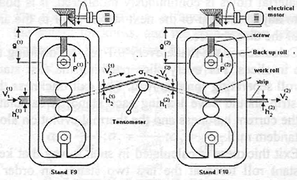
Fig. 1: Rolling mill stands escheme

These rolls drag the strip to the Stand roll bite, reducing its thickness. This strip has to leave the actual stand and enter in the next until the desired thickness is reached and is coiled in the output of the last Stand.

The main motivation of this work is the reduction of the output thickness variations of any of two input process variables disturbance: strip temperature and input strip thickness. Fig. 2 shows three graphics of real rolling mill process. In Fig. 2 (a) we observe the rolling force and the cold zones indicated by arrows, that are due to skid marks at the furnaces. In Fig. 2 (b) we can see the temperatures and in Fig. 2 (c) the consequent exit thickness.

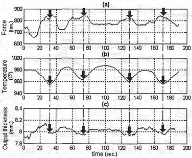
Fig. 2: Strip cold points.

These cold zones have greater deformation resistance and increases the rolling mill force in the stand. This variations in the rolling mill force produce variations in the stand stretching, leading to variations in the output strip thickness at the stand.

Observing the output temperature of the rolling mill stand, it can be seen low temperature zones that are the skid marks previously mentioned. On the other hand, from the beginning to the end of the process a decreasing temperature is observed. This thermal lose produces a proportional increasing in the rolling force and in the output strip thickness as presented in Fig. 2 (c), being the temperature variations and the input thickness the mainly responsables of the variations in the rolling force altering the output strip thickness .

II. CONVENTIONAL CONTROL - FORCE FEED FORDWARD (FFF)

The force feed-forward (FFF) thickness control technique is based in the detection of hardness fluctuations in the material as it passes through the first finishing stand, and the data sent from the setup model.

Keeping the gap constant at that stand, differences in hardness are reflected as roll force variations. Therefore, if material flows is continuously monitored, it is possible to adjust the gap of the next stands prior to the arrival of the disturbance.

Calculations are made every 0.1 sec. by dividing the strip in slices. For every slice reaching the first stand, the roll separating force is read. The exit thickness that the strip should have leaving each stand, is calculated for the current hardness and the thermal evolution along the tandem mill.

Exit thickness is calculated in such a way that keep constant roll force at the last two stands, in order to avoid affecting strip shape. Since the temperature of the material at the last stands is known the entry thickness to them are evaluated in a way that thinner thickness correspond to colder slices and vice-versa.

Thickness in the intermediate stands are computed to maintain load distribution defined by the setup model. Once thickness and temperature at each stand have been determined, roll force can be calculated.

For every slice is calculated the same set of data and stored in the control computer memory buffers. The tracking of the slices as they flow through the stands allows the system to know their current location. Gap and a roll speed adjustments are defined for the slice that is to reach any given stand at the time that equals mill drivers response time.

Deviations measured at the thickness gage are used to make a fast correction at the last stand and calculation adjustments are done in order to keep the previous load distribution.

The FFF scheme is shown in Fig. 3.

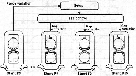
Fig. 3: Force Feed Forward Control

III. PROPOSED CONTROL

In order to develop the control law in the last two Stands we applied optimal control techniques with integral action on the model represented in state space formulation. Fig. 4 shows the proposed control scheme.

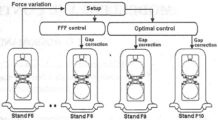
Fig. 4: Proposed Optimal control in the last two stands.

For the considered system our control inputs are Δg_in⁽¹⁾, ΔV_in⁽¹⁾, Δg_in⁽²⁾, the controlled outputs are Δh₂⁽¹⁾, Δσ₁, Δh₂⁽²⁾, and the measured outputs are Δh₂⁽¹⁾, Δσ₁, Δh₂⁽²⁾, ΔP^{(1) y} ΔP⁽²⁾. The main control objective is to maintain the strip output thickness variation (Δh₂) closer to zero, for any temperature or strip input thickness variation in the system.

All input variable deviation is considered a disturbance and the control system should maintain the thickness variation closer to zero acting on gap variation (Δg_in), which is our control variable of the output thickness variation (Δh₂).

Similar actions are taken for tension variations which depends on the amount of strip accumulated between the last two Stands F9 and F10. This tension is a function of the difference between the strip output and input speeds on the Stands F9 and F10 respectively. In our case this tension is controlled by the rolls tip speed variation of the Stand F9.

In this case, in literature one can find successful applications of linear MIMO-(multi-input multi-output) controllers to multi-stand rolling mills, which, in fact, overcome the deficiencies of the classical single-loop control concepts ,see, e.g., Grimble and Hearns (1998) and Hoshino et al. (1988).

A. Analytical Process Modeling

In this work we presented a mathematical model for the last Stands F9 and F10 of the tandem rolling mill, to evaluate the proposed control technique. (FFF system makes the thickness adjustment in the last two Stands), the analytical model used is for the validation, by simulation, of the results obtained.

Those results are compared with real values measured in the rolling mill stands controlled by the FFF technique. (Bryant, 1973; Ginzburg , 1989).

To obtain an approximated rolling model, we worked with Orowan and Alexander theories (Orowan, 1944; Alexander, 1972), which appears more reliable to obtain the rolling mill force, being able to be used in a wide set of conditions of strip rolling. The mathematical model was fit and calibrated with values measured in real process, getting a closer response to the real force value, this model is represented in a general form by Eq. (4) and the sliding by Eq. (5).

B. Basic model equations

The implemented mathematical model considers the last two rolling stands, since FFF control makes the thickness adjustment in the preceeding ones. In our case we make the thickness adjustment by optimal control technique, using the mathematical model expressed in the state space form. The output thickness of each Stand is a function of the rolls gap and the stand streching

(1)

where:

(i) :	Rolling mill stand i=l (F9), i=2 (F10).
h2(i) :	Output strip thickness of the stand (i).
g(i) :	Rolls gap of the stand (i)
P(i) :	Roling mill force of the stand (i).
K(i) :	Elasticity Modulus of the Stand (i).

The derived strip tension between the Stands is a function of the difference between the strip output and input speed on Stands F9 and F10:

(2)

where:

σ1 :	Strip tension between stands F9 and F10.
E :	Strip Young modulus 21.000 N/m
L :	distance between Stands (i). 5.486 m.
V2(1) :	output strip velocity of the Stand F9.
V1(2) :	input strip velocity of the Stand F10.

The volume continuity of the strip in the rolls gap is defined as

V₁⁽ⁱ⁾ h₁⁽ⁱ⁾ = V₂⁽ⁱ⁾ h₂⁽ⁱ⁾. (3)

The rolling mill force is resented by Eq. (4).

P⁽ⁱ⁾ = P(h₁⁽ⁱ⁾, h₂⁽ⁱ⁾, σ₁⁽ⁱ⁾, σ₂⁽ⁱ⁾, S⁽ⁱ⁾, μ⁽ⁱ⁾, T⁽ⁱ⁾), (4)

where:

σ2(i) :	output strip tension on the Stand (i)
g(i) :	rolls gap for the Stand (i).
μ(i) :	friction Coeficient on the Stand (i).
S(i) :	Yield stress on the Stand (i).

Sliping function is defined like:

f⁽ⁱ⁾ = f(h₁⁽ⁱ⁾, h₂⁽ⁱ⁾, σ₁⁽ⁱ⁾). (5)

C. Model basic considerations

i) The main consideration is that the control is applied when a strip exists between both stands, this means, that the previous moment to the entrance of the strip in the last stand is not considered.

ii) We considered the finite variations of the nominal values. For example variable x, being Δx the finite variation and x^* the nominal value.

iii) We have also considered that the rolling force is a function of the input thickness, output thickness, strip temperature and strip tension between Stands (Pedersen, 1995; Denti, 1994; Hoshino et al., 1988). The sensitivity curves show the rolling mill force variation:

(6)

The coefficients of the linear functions are:

(7)

iv) The sliding variation is a function of the input and the output thickness, and the strip tension which is represented by equations (8) and (9).:

(8)

The coefficients are:

(9)

v) The strip output speed variation is expressed by the sliding variation coefficients and by the roll tip speed:

(10)

vi) The controlled variables are not affected directly by the tip speed of the last stand. Then we have ΔV₂=0.

vii)Each actuator has its own dynamic that can be- approximated by a first order system expressed as:

	(11)
	(12)

viii) The variables Δhl⁽¹⁾ ΔT⁽¹⁾ and ΔT⁽²⁾ will be considered as system disturbances;

ix) Considering the transport delay between F9 and F10, the output strip thickness variation on the Stand F9 is equal to the input strip thickness variation on the Stand F10. The delay time is equal to Td=L/(V+ΔV) then Δh₂⁽¹⁾=Δh₁⁽²⁾.exp(-s.Td). where s is the Laplace operator.

The general model structure represented in the state space is shown in equation (13)

(13)

where the input, states, output and disturbance vectors are:

The coefficients needed to generate the state space matrixes are:

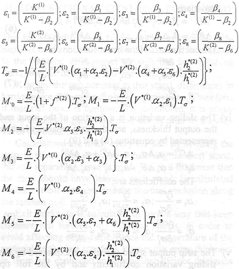
The matrixes A, B, C, F, E₁, E₂ and E₃ are:

The previous model is converted to discrete time state space with sample time of t_o=0.1 seg.

(14)

To demonstrate that the process is totally controllable we construct the controllability matrix M_c (Kuo, 1992; Ogata, 1996; Grimble et al., 1998; Kuchen et al., 2000).

(15)

We obtained that the matrix rank M_c is equal to the process order demonstrating that it is completely controllable. In order to prove that the system is completely observable, this is, if the state vector can be determine from the measurement of the output vector during a finite time interval, we define matrix M_o as:

(16)

Where M_o matrix rank is equal to the process order, that confirm it is completely observable.

For the controller design we look for a state transition matrix to obtain the best possible process response with addition of an integral action to reduce the process stationary state error.

The inclusion of the integral action increases the system order, if the system is of 4th order and the number of feedback variables with integral action is 3 then, the new system order is 7 (4+3) and the new state vector for the calculus of the optimal integral regulator will have a dimension equal to 7 (4+3).

To this new extended order, the considered model is still observable and controllable. The new state vector can be defined as ξ(k) = [x(k) v(k)]^T, being vector v(k) the integral action for the three feedback variables. The new matrixes A and B are

The performance index proposed for integral optimal controller is:

(17)

The two matrixes R and Q are symmetrical positive definite and our objective is to find the optimal value for the index J. The plant structure is the established in the state space, and the calculation of the controller gain matrix must be done offline, by the Riccati equation. The Riccati equation , for the stationary state is:

(18)

From the value of the gain matrix K is.

(19)

With the gain calculated in the Eq. (19), being = [K - K_i] then the control law is:

(20)

The optimal control block diagram is shown in Fig. 5, where it is assumed that all the states are available. The eigenvalues of Eq (21) must be inside of unit circle. With the state feedback the system is autonomous, where the system dynamic is governed by the eigenvalues matrix as it is shown in Eq (21):

(21)

The eigenvalues of the system with the optimal controller or with the optimal controller with integral action lies inside the unit circle.

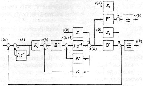
Fig. 5: The Optimal model control represented in state space.

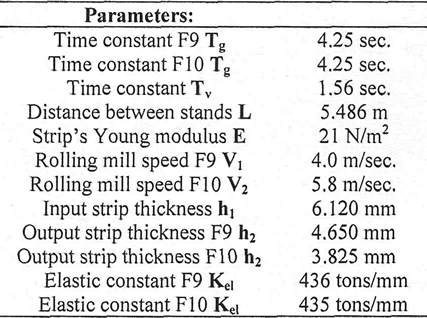
Where the reference vector is r(k)=[0,0,0]^T. The Table 1 indicates the model parameters used in this article.

Table 1: Model parameters

D. Control Results Validation

In order to make the control technique evaluation, it was collected real rolling mill data of the steel coil, with N^o 982 1612 rolled in the SIDERAR S.A. plant in Argentina.

Fig. 6 shows the measured input thickness variation , the temperature process variation of the real rolling mill that are applied to the model to test the proposed control law. Only variations concerned with the operation point were introduced. Simulation results show the output thickness variations (Δh₂⁽¹⁾ and Δh₂⁽²⁾), the strip tension variations (Δσ₁), and the control action for both Stands (Δg⁽¹⁾ ΔV⁽¹⁾ Δg⁽²⁾). The control results for an optimal controller and for an optimal controller with integral action are shown in the next figures.

Fig. 6: Strip thickness and temperature Variation of Stands F9 and F10.

Fig. 7 shows the output thickness variations for Stands F9 and F10, being the output expected reference variation equal to zero. The optimal control error is lower than 30 um and in the case of conventional control (FFF) it goes up to 100 |am. The same results for different data collected in the rolling mill process were obtained and the thickness error in the case of the optimal control is always smaller than the error of the control FFF, which is the real controller used in the plant.

Fig. 7: Strip output thickness Variation of Stands F9 and F10 with FFF, optimal control and optimal control with integral action

Fig. 8 shows the gap variation in the Stands to compensate model disturbances. Fig. 9 shows the strip tension calculated by the simulation model, the real strip tension variation is not well-known and was estimated based on looper angle.

Fig. 8: Gap variation of Stands F9 and F10 respectively.

Fig. 9: Strip tension variation and speed control variation of Stand F9.

The last figure (Fig. 10) shows simulation results for the rolling force for a FFF control and optimal control

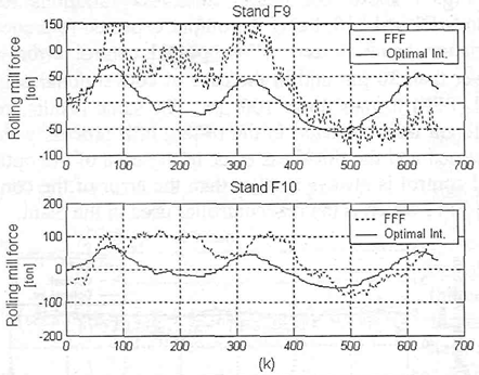
Fig. 10: Rolling force variation with integral optimal control for Stands F9 and F10 respectively.

It is important to note that the control objective is the output thickness (Fig. 7). In Fig. 9 and Fig. 10 we observe the efects in interstands tensions and in the rolling force as a consequence of the control action.

IV. CONCLUSIONS

The rolling mill model presented in this article is calibrated with real values measured in a real rolling process and constructed with parameters provided by Siderar S.A. company

Later, having the linear model around the operation point we obtain a state space model representation. In this way we have a dynamic model for the last two rolling stands with a behavior too similar to the real process within the operation range that was considered.

The results shows the thickness variation of the two control techniques. The optimal control technique of the process evaluated by computational simulation, show an smaller thickness variation than the real system force feed forward FFF, that was take for comparison, FFF presents a greater thickness dispersion than the optimal controller.

The technique is simple to implement and could be used in parallel, for performance verification in real operation conditions , allowing a possible substitution of the system force feed forward (FFF) in the future in last two rolling mill stands.

REFERENCES
1. Alexander, J.M., "On the Theory of Rolling"; Proc. R. Soc. London, A. 326, 535-63 (1972).         [ Links ]
2. Bryant, G.F., Automation of Tandem Mills; London, The Iron and Steel Institute, Publication No. 160, (1973).         [ Links ]
3. Denti Filho, J., Un método de Controle Dinâmico de Laminadores reversíveis, UFMG (1994).         [ Links ]
4. Ginzburg, V. Steel Rolling Technology: Theory and Practice. Marcel Dekker. New York and Basel (1989).         [ Links ]
5. Grimble, M.J. and G. Hearns, "LQG Controllers for State-Space Systems with Pure Transport Delays: Application to Hot Strip Mills", Automatica, 34, 1169-1184 (1998).         [ Links ]
6. Hoshino, I., Y. Maekawa, T. Fujimoto, H. Kimura and H. Kimura, "Observer-based multivariable control of the aluminium cold tandem mill", Automatica, 24 , pp 741-758 (1988).         [ Links ]
7. Kuchen, B., R. Carelli, J. Postigo and V. Mut, Control Digital Avanzado, Reporte interno Instituto de Automatica, UNSJ (2000).         [ Links ]
8. Kuo, B., Automatic Control Systems. Prentice Hall Inc, fourth edition. (1992).         [ Links ]
9. Ogata, K., Modern Control Engineering. Prentice Hall Inc, third edition. (1996).         [ Links ]
10. Orowan, E., "The Calculation of Roll Pressure in Hot and Cold Rolling"; Proc. Inst. Of Mechanical Engineers, 150, 140-167 (1944).         [ Links ]
11. Pedersen, L., Modeling and identification of hot rolling mill. In proc. of the American Control Conference. 3674-3680 (1995).         [ Links ]

Received: March 2, 2006.
Accepted: May 23, 2006.
Recommended by Subject Editor A. Cuitifio.