Predictive control with constraints of a multi-pool irrigation canal prototype

O. Begovich¹, V. M. Ruiz², G. Besançon³, C. I. Aldana¹ and D. Georges³

¹ Centro de Investigación y Estudios Avanzados, Unidad Guadalajara, A.P.31-438, Jalisco, México
obegovi@gdl.cinvestav.mx
² Instituto Mexicano de Tecnología del Agua, 62550, Jiutepec, Morelos, México
vmruiz@tlaloc.imta.mx
³ Laboratoire d'Automatique de Grenoble, INPG - CNRS, BP 46,38402 Saint Martín d'Héres, France.
Gildas.Besancon@inpg.fr

Abstract — This paper presents a real-time implementation of a multivariable predictive controller with constraints to regulate the downstream levels at the end of the pools in a four-pool open irrigation canal prototype. The objective of the controller is to maintain the downstream level at a constant target value despite inflow disturbances. The controller is designed using a "black box" identified linear model. The results show satisfactory closed-loop performances.

Keywords — Predictive Control. Automatic Control. Control Applications. Hydraulics. Identification.

I. INTRODUCTION

In many countries open irrigation canals are used for the distribution of water in agriculture. In general the control structures on the canal are manually driven with poor efficiency results. In our days, the best alternative to improve distribution efficiency and operation of irrigation canals is the use of automatic control structures. The main goal in canal operation is to supply the water flow rate to farmers in quantity and frequency.

The present work is related to a real-time application of an automatic control in open irrigation canals. The automatization of such systems is not simple, since: the dynamics of water through the canals are modeled by nonlinear partial differential equations (Saint-Venant equations); they have a lot of inputs (typically gates) as well as outputs to be regulated (basically the levels); the dynamics of the water flow are characterized by delays between a control action and its effect on the levels along the canal, and they are subject to disturbances, which are mainly due to water withdrawals or weather conditions.

A variety of methods have been proposed in order to deal with the problem of automatic control for canals. These works range from classical PI (Mareels et al., 2005; Malaterre et al. 1998; Ruiz-Carmona et al., 1998) to advanced controllers handling partial differential equations (Chen and Georges, 2001) or nonlinearities (Dulhoste et al., 2004). Model Predictive Control (MPC) strategy has also been considered by Rodellar et al. (1993) where a monovariable input/output model is used to design a predictive controller in order to control a single reach of canal. In Malaterre and Rodellar (1997) or Pages et al. Sau (1997), centralized multivariable controllers for canal automation are derived based on predictive control techniques. In Sawadogo et al. (1998) a decentralized predictive controller is developed. A recent and interesting work in MPC applied to irrigation canals is found in Wahlin (2004). In that work an MPC is tested in a Benchmark canal, the "ASCE Test canal 1" (Clemmens et al., 1998). This canal is an eight-pool trapezoidal canal. The model used to design the MPC is the model called the "integrator-delay" (ID) (Schuurmans et al., 1995). The MPC designed is tested under scheduled and unscheduled flow rate. For the case of the scheduled flow variations, a feedforward controller is also considered. In some tests realized in that paper, the minimum gate movement of the control gate is set to zero when the opening gate is less than a minimum specified value. The level performance is satisfactory when the gate opening is not constrained, but it decreases when it is constrained.

In all these works, the performance of the closed-loop (canal/controller) is tested only in computer simulation but not in any physical canal. As far as we know, no application of a predictive control to regulate some real irrigation canals or canal prototypes has been reported so far¹.

In this paper we present the design and real-time implementation results of a recent centralized Model Predictive Control algorithm (MPC) (Maciejowski, 2002) for a four-pool open canal prototype that takes into account operational constraints (e.g. bounds in control actions and output variables) to regulate the downstream levels of each pool. The model used to design the MPC is a transfer matrix obtained by identification. The control actions are calculated by an optimizer taking into account a cost function where the future tracking error is considered together with the operational constraints (Maciejowski, 2002; Camacho and Bordons, 1999). Since the MPC technique is capable to handle system constraints and delays, as those existing in long canals, this work aims at evaluating the perfor-mance obtained with this algorithm and at assessing the easiness/difficulty as well as the required equipment to implement this kind of algorithms in some real irrigation system.

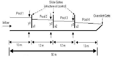
The canal considered in this paper is represented in Fig. 1, here the controlled variables are the downstream levels of the first three pools and the control variables are the openings of the slide gates along of the canal. At the head of the canal, a servo valve drives inflow disturbances. The considered pool operation method and control concept are constant downstream level and upstream control respectively (Buyalski et al., 1991).

(a)

(b)
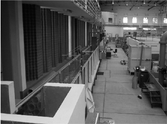
Fig. 1. (a) Irrigation canal prototype scheme, (b) Irrigation canal prototype photo

This paper is organized as follows. In section II, the characteristics of the laboratory canal which is used are presented. In section III, the methodology to obtain a "black box" linear input-output model is given. In section IV, the synthesis of the proposed Model Predictive Controller is described. Section V shows some real-time results from the closed-loop system. Finally, the conclusions are stated.

II. FOUR-POOL LABORATORY CANAL

For this application a zero slope rectangular canal with glass walls and concrete bottom, of 60 cm wide, 50 m long and 1 m high, available at Mexican Institute of Water Technology (IMTA) laboratory is used. As control structures, three slide gates are installed and they divide the canal into four pools, see Fig. 1. The inflow is adjusted with a servo-valve. At the downstream end of the canal the level is regulated by a manual overshot gate.

Each slide gate is equipped with a linear actuator, two pressure sensors (upstream and downstream), a potentiometer for gate position and limit switches (maximum and minimum gate opening). The flow regime through the slides gates is submerged with gate influence (Chow, 1988). This prototype does not have any lateral outlets

The system is designed considering manual operation and RTU (Remote Terminal Unit) operation. The RTU operation can be remote manual operation or local automatic operation. The RTU which is used is a MODICOM PLC E984-245 at gates 2 and 3, and a SCADAPack from Control Microsystems at gate 1. A Pentium PC is used as a master station where the man-machine interface was installed using Lookout software from National Instruments Inc. The master station is relayed by radio to the SCADAPack (MODBUS protocol) and by wire to the PLC (MODBUS+ protocol).

III. MODEL

In open irrigation canals the water dynamics are modeled by two nonlinear partial differential equations named the Saint Venant equations (Chow, 1988). This model is used to study the level and flow behavior, but in general, it is not used for control design due to its complexity. Instead, several authors propose simple models such: state-space linear models obtained by discretization of the Saint Venant's equations (Malatererre and Rodellar, 1997), state-space nonlinear models (Besançon et al., 2004), input-output (I/O) nonlinear models (Euren and Weyer, 2005) or I/O linear models (Begovich, 2005), for example.

In this section a simple input-output linear model is obtained by identification, and it will be used to design an MPC controller. The proposed linear model is a transfer matrix and the identification is carried on to estimate the parameters of the transfer functions, entries of the transfer matrix. These transfer functions approximate the water dynamics. Identification follows the next procedure (Ljung, 1987):

A. Selection of input and output variables.

In an irrigation canal, the control action can be the gate opening or indirectly the flow through the gate. If the control variable is considered to be the flow, a second control loop (slave) is usually required in order to maintain the flow when the level upstream and/or downstream the gate is changed. The main advantage in using the flow as a control variable is to reduce the cross-coupling interaction between the controlled pools in a canal, which can be of particular interest when a decentralized control is projected. Looking for the simplest solution that could actually be implemented on some operating canal, we rather choose the gate opening as the control variable for the prototype as well as the actual application carried on at the Colorado River irrigation district in Mexico. The use of flow as control variable and downstream control concepts is under study.

Moreover, although the choice of gate opening as a control variable does not reduce the cross-coupling interaction in the same way as the inflow control action can do, the cross-coupling interaction remains quite small in our case and a successful decentralized control can still be implemented in real time as shown in Begovich (2007).

On the other hand, the output variable is usually considered to be the level at the downstream end, since it is there that one generally finds the outlets when the farmers take water from the canal. Maintaining constant this level can thus guarantee a constant flow for the users. This is the situation indeed found in Mexican canals, and for this reason the downstream level of each pool is selected here as the output variable (variable to be controlled).

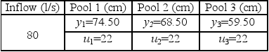
Summarizing, the input variables are selected as the opening deviations from the set point of the gates located at the downstream end of the pools. They are denoted by: u_i (i=1, 2, 3), where i is the i-pool. The output variables are the level variations at the downstream end of the pools. They are denoted by y_j ( j = 1, 2, 3). The linear model will be identified around the set point given in Table 1.

Table 1. Canal set point

B. The Data.

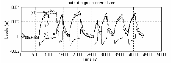
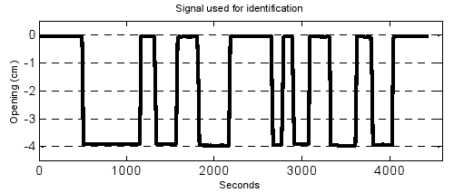
During the second phase, the variations in the water level y_j (j=1, 2, 3) are registered when we apply a binary signal of random duration: first on gate 1, next on gate 2 and finally on gate 3, see Fig. 2d. The amplitude of this signal is of the 20% with respect to the set point of each gate. The fast changes in the binary signal ensure that this signal has a large bandwidth. In this way, the most significant canal frequencies will be excited and a good parameter identification will be achieved. The order of frequencies in this canal is 10^-2 rad/s, and the time constants range from 70s to 120s (Begovich et al., 2002).

(a)

(b)

(c)

(d)
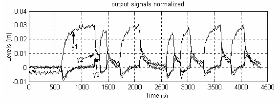
Figure 2. Levels registered (y₁, y₂, y₃) when the binary signal in (d) is applied only to (a) first gate (b)second gate (c) third gate (d) input binary signal

To register the data, in this experiment the sample time was chosen equal to 10 seconds, since this value represents a good compromise between acceptable opening gate rates and an accurate rebuilding (Shannon's Sampling Theorem). In Fig 2 the downstream levels evolutions obtained are presented. Notice that the signals are normalized with respect to each respective set point (see Table 1).

C. Proposed model.

From Fig. 2, it is observed that downstream level responses are very similar to those of linear systems, and that is why we propose the following structure:

y(z) = H(z)u(z) (1)

where

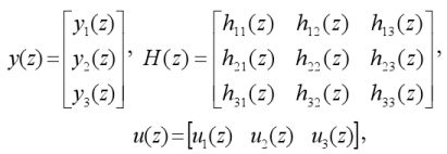(2)

h_ij represents the transfer from u_j to y_i. Each h_ij is estimated through the identification of an output error model structure (Ljung, 1987)

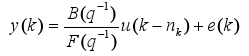(3)

where

(4)

are polynomials in the shift operator q^-1, n_k are the delay, n_b and n_f are the orders of polynomials B and F respectively, e is the residual, and k is the discrete time.

D. Parameter estimation.

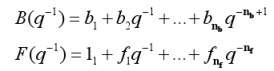
To estimate the values of coefficients b_i and f_i, in this work we use the instruction oe (output error) of the Matlab System Identification toolbox. The values of n_k, n_b, n_f being determined by optimizing some corresponding performance index within the toolbox facilities (via the function compare). As soon as the output error models are obtained for each couple of data (u_j, y_i), they are expressed as transfer functions, finally giving:

(5)

It can be noticed that the order of the obtained transfer functions is two or three. This is specifically due to the fact that the model is here obtained directly by identification. This identification captures the gate and actuator dynamics (since the input variable is gate position instead pool inflow) and the small delays of the considered prototype. These effects are approximated in the interpolation carried out by identification and result in the respectively obtained orders. Models of similar order could be obtained from those of Mareels et al. (2005), or Clemmens and Schuurmans (2004) for instance, if delays were approximated by some expansion, such as Pade expansion.

E. Validation.

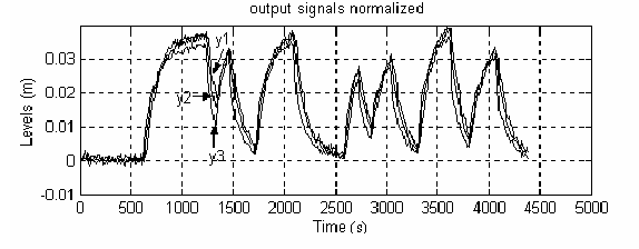
To verify the model accuracy, the measured outputs of the actual canal system are compared with the outputs of the identified model, when the same input is applied to both systems. This comparison is shown in Fig. 3, where it can be seen that the model responses (dotted lines) indeed follow the measured ones (solid lines).

Fig. 3. Comparison between measured system outputs and the model responses [H₁₁ H₁₂ H₁₃; H₂₁ H₂₂ H_23; H₃₁ H₃₂ H₃₃] when the same input is applied to the system and the model

F. State-Space Representation.

To design the predictive controller, the transfer matrix representation is transformed to a state-space representation. To do that, first we obtain the state space of each transfer function in (5). After we use all the individual realizations to obtain the state space realization of the matrix transfer following the more simple methodology stated in Kailath (1980). Finally, the realization obtained needs to be transformed into a minimal one (i.e. a realization that is controllable and observable) for its use in the controller design. This can be done with functions tf2ss and minreal from the Control Toolbox of Matlab. The representation which is finally obtained is denoted by:

x(k+1) = A_px(k) + B_pu(k)
y(k) = C_px(k)

where x is the state, u is the input vector, y is the output vector, and A_p, B_p, C_p, are matrices of appropriate dimensions. In practice the dimension of the obtained observable and controllable realization was n=20. Values of A_p, B_p, C_p, are omitted due to space limitation, but they can be found in Aldana (2004). This reference is available from the authors via e-mail.

IV. CONTROLLER SYNTHESIS

A. Preliminaries on Predictive Control

Predictive control uses an available system model to incorporate the predicted future behavior of the process into the controller design procedure. This method of control design usually combines: 1) A process model; often a linear discrete one 2) A predictor equation; this is run forward for a fixed number of time steps to predict the likely process behavior 3) A known future reference trajectory 4) A cost function; this is usually a quadratic function which penalizes future process output errors with respect to the known reference and control values. Optimizing the cost function subject to future process outputs and controls leads to an explicit expression for the control. One further capability of the method is that it can incorporate operational process constraints. If these constraints are given in linear inequality form, the optimization problem in the predictive control takes the form of a Quadratic Programming (QP) problem which can be solved using standard methods of optimization.

B. MPC Algorithm.

In this work, the following predictive control algorithm incorporating operational process constraints (Maciejowski, 2002) is used: For the process model

x(k+1) = Ax(k) + Bu(k)	(6)
y(k) = Cx(k)

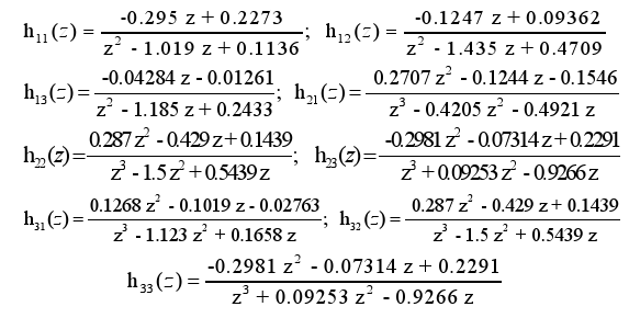
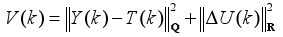
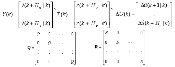
the cost function is settled as

(7)

where

H_p: Prediction Horizon; H_w: Beginning of prediction horizon; H_u: Control Horizon;

r(k+i|k): Future value at time k+i of the reference trajectory, which is assumed at time k

Δû(k+i|k): Future change of the input u, which is assumed at time k;

Q_i≥0 and R_i>0 are diagonal weighting matrices that penalize the differences between the outputs and references, and the changes in the input vector respectively. In this work Q_i =Q and R_i =Ri, i.e. the weighting matrices are constant matrices on the considered horizons.

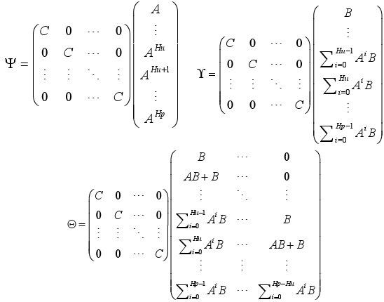
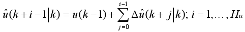
The predictor equation is given as:

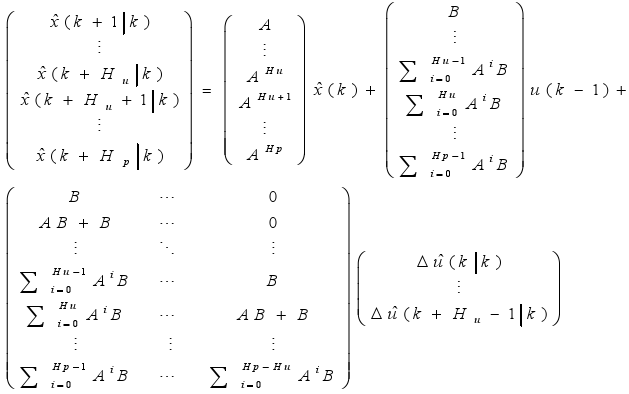(8)

where (k) is the estimated state.

The predictions of the outputs are obtained as:

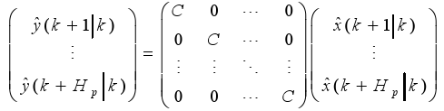(9)

For convenience the cost function (7) is rewritten as:

(10)

where

substituting (8) in (9), we get

(11)

where

Now define E(k) as:

(12)

this equation represents the difference between the future target trajectory and the response that would occur over the prediction horizon if no input changes were made, i.e. if ΔU(k)=0.

Using (11) and (12) in Eq. (10), the cost function can be rewritten as:

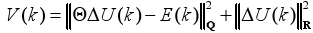(13)

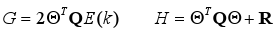
(14)

where:

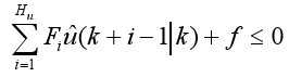
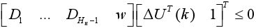
The present predictive control algorithm assumes that the constraints over outputs, inputs and actuator slew rates are represented in the following form:

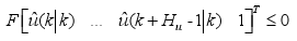	(a)	(15)
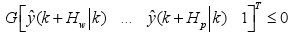	(b)
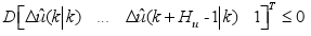	(c)

where D, F, G are matrices whose values are obtained when the restrictions are taken to the form of (15). Note that equation (15a) represents actuator constraints, (15b) output constraints and (15c) constraints over actuator slew rates.

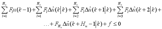
Since the cost function (13) is minimized with respect to ΔU(k), the constraints (15a) and (15b) must be rewritten, to express them as constraints of ΔU(k) as follows:

(a) To express (15a) as a function of ΔU(k), F is divided as follows:

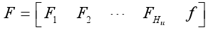(16)

where each F_i is of size q × m (q number of restrictions on u and m dimension of u) and f is the last column of F, so that (15a) can be written as:

(17)

but

(18)

and combining (17) with (18) yields:

(19)

Now define

(20)

Using (20) in (19), we have that (15a) can be expressed as a function of ΔU(k) as:

FΔU(k) ≤ -F1u(k-1) - f (21)

(b) Note that (15b) is equivalent to G[Y^T (k) 1]^T ≤ 0, then using (11) this constraint is written as:

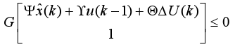(22)

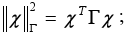
Now writing G as G = [Γ g], where g is the last column of G and Γ the matrix composed by the other columns of G, then (22) is expressed as:

(23)

(c) Finally, if in (15c) D is divided into 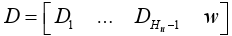, where each D_i is a q × m matrix, i=1,...,H_u-1 and w is the last column of D, this equation can be written as

(24)

defining 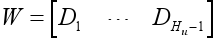, equation (24) results in

WΔU(k) ≤ w (25)

Then, inequalities (21), (23), and (25) are gathered into the following single inequality:

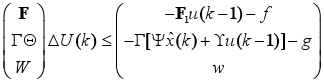(26)

Therefore, the solution to this predictive control problem consists in the minimization of (14) in relation to ΔU(k), subject to the inequality constraint (26). This is a standard QP optimization problem and standard algorithms can be used for its solution.

The control law is used in the receding horizon sense, i.e., at each sample time only the first m (where m is the control variable vector dimension) elements of ΔU(k) are used, i.e.

Δu(k)_opt = [I_m 0_m ··· 0_m]ΔU(k)_opt (27)

where I_m is an identity matrix and 0_m is a zero m × m matrix.

C. Disturbance Model and Disturbance Rejection

In irrigation canals, the main sources of disturbances are: implementation of a new distribution irrigation schedule, user withdrawals and weather variations, and they have influences on the pool levels observed as constant disturbances in steady state. Thus, these disturbances can roughly be modeled as step variations. In our prototype, there is no withdrawal, but inflow variations at the head of the canal can be produced as disturbances, and such variations propagate to the downstream pools, modifying their inflows, and then their downstream levels, under the form of constant disturbances.

In Control Theory it is well known that the internal model producing a constant disturbance is an integrator (Ogata, 1991) and from the Internal Model Principle (Wonham, 1985) that in order to reject a constant disturbance it is necessary that an integrator (i.e. the internal model of the constant disturbance) appears in the open loop transfer function. From the above discussion, we can propose as internal model of canal disturbances an integrator for each pool, and it is expressed as

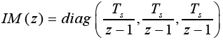(28)

where T_s is the sampling time.

To satisfy the Internal Model Principle, the controller will be designed using the augmented linear model, i.e. the identified linear model of the canal (2) and (5) plus the internal model of the disturbances (28). The state space realization of this augmented plant was obtained as a serial connection between the linear model realization and the realization of the internal model of the disturbances resulting into the next state model representation:

x(k+1) = Ax(k) + Bu(k)	(29)
y(k) = Cx(k)

Now x represents the sate of the augmented plant. Values of A, B, C, are omitted do to space limitation, but they can be found in Aldana (2004).

The interested reader can verify that the previous internal model is also efficient to model withdrawals as shown in Begovich et al. (2005).

D. Specifications

The closed-loop canal must satisfy the following specifications to guarantee the supply to the consumers, to avoid water spillage, and to protect the control structures:

• Level variations must be less than 15% with respect to the level of the operating points.
• The gate-opening rate should not exceed 1 cm/s.
• The gate-opening rate should not exceed 1 cm/s.
• The gate-opening limit is 80 cm.

Expressing the last specifications as operational constraints, results in:

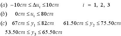(30)

E. Design of the Predictive Controller

The predictive controller design is based on the algorithm described earlier. Next we mention the requirements of the algorithm that could be done offline, and then summarize the steps followed by the algorithm at each sampling time.

Requirements:

Sampling time k: chosen equal to 10 seconds.

I/O data: vector of levels y(k); vector of control gate positions u(k); vector of level references r(k).

Model: the augmented model (A,B,C) given in (29).

Synthesis parameters: given in Table 2.

Operational constraints: given in (30) and their transformation into the inequalities (15).

Estimation(k): given by a deadbeat observer (Åström and Wittenmark, 1997).

The steps followed by the algorithm at each sampling time are:

1. Updates of the vectors of levels y(k), and inputs u(k).
2. Estimation (k) from the observer using the information (y(k), u(k)).
3. Prediction of Y(k) by implementing the equations (8) and (9).
4. Generation of T(k), ΔU(k)
5. Update of the constraint matrix of inequality (26)
6. Minimization of (14) subject to (26) using a QP algorithm.
7. Implementation of the control law Δu(k)_opt using the receding horizon strategy.

In this work, the transformation of the operational constraints in (30) to the form needed for the algorithm follows the procedure cited in Ch. 2 of Maciejowski (2002), this transformation as well as the observer and predictor are programmed in Matlab. The minimization of (14) subject to (26), is developed using the function dantzgmp of Matlab.

The real-time implementation is carried out with Lookout software to get and deliver information from/to the process. This information is used by Matlab for the iterative calculation of the control algorithm at each sample time.

V. EXPERIMENTAL RESULTS

The following experiments were carried on the laboratory canal described in Section 2. The operating points are stated in Table 1; the sample time is 10 seconds and the disturbances are step variations on the nominal inflow (80 l/s). The control design is tested with the synthesis parameters showed in Table 2, where I is the identity matrix.

Table 2. MPC Synthesis parameters

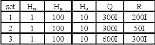
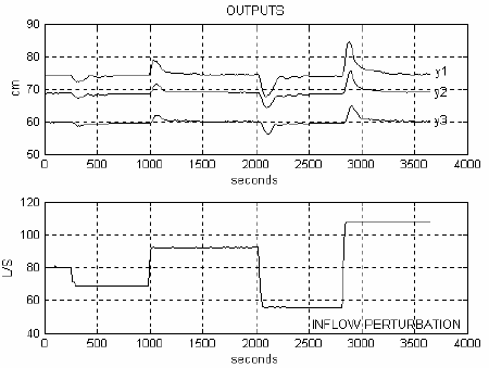
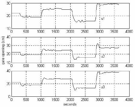
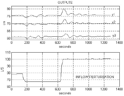
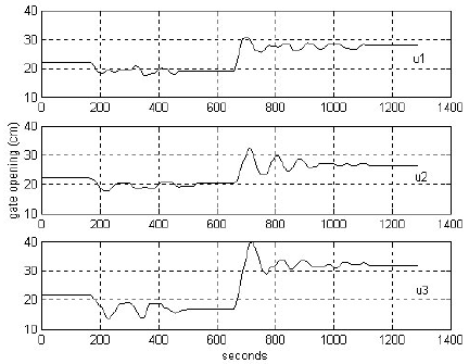
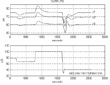
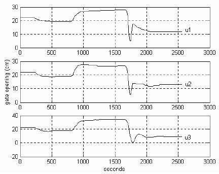
Figure 4, Fig. 5 and Fig. 6 show the downstream level responses (outputs) and the MPC control laws, when inflow disturbances act on the canal. The results of Fig. 4 are obtained when the first set of parameters showed at Table 2 is used. As it can be seen in Fig. 4, a good compromise between speed in the disturbance rejection and smoothness in the control variables is obtained. In Fig. 5, the second group of parameters of Table 2 is tested. Faster disturbance rejection is presented but control variables are more demanded. In Fig. 6, the last group of parameters gives very smooth control law and not too fast disturbance rejection. In the three cases, adequate regulation of the downstream levels in presence of the input flow disturbances can be seen. Furthermore, the gate openings do not exceed their physical limits, and the opening-rate remains below the specified maximum one. In general, an adequate performance is obtained in the closed-loop system. Moreover, from those experiments it can be seen, in a qualitative sense, that the characteristics of first and third groups of parameters are good options for a future MPC application in an irrigation canal in field.

(a)

(b)
Fig. 4. Closed-loop system responses, when the predictive controller is designed using the first set of parameters in Table 2: (a) Levels and the inflow disturbance (b) Predictive control laws

(a)

(b)
Fig. 5. Closed-loop system responses, when the predictive controller is designed using the second set of parameters in Table 2: (a) levels and the inflow disturbance (b) Predictive control laws

(a)

(b)
Fig. 6. Closed-loop system responses, when the predictive controller is designed using the third set of parameters in table 2: (a) Levels and the inflow disturbance (b) Predictive control laws

The inclusion of restrictions in the design allowed to satisfy easily the specifications, but as a counterpart, the algorithm is more complicated than an MPC without such restrictions. In our case, implementation in real-time of this algorithm was relativity simple due to the use of a central computer and programs like Matlab and Lookout. However, in many operational canals in irrigation districts only PLC's or SCADA systems are available. Then, an interesting future work is to evaluate the difficulty to implement the proposed algorithm in this context. Such implementation is indeed attractive due the potential capacity to manage long delays and constraints which are significant in those systems.

Even if in our prototype, delays are in fact quite small, this work has allowed to evaluate in real-time: the problem of implementation of the proposed algorithm, its regulation performance and its capacity to handle constraints.

The interested reader can for instance consult references Begovich et al. (2002) and Begovich, et al. (2005) to compare the performances here presented to those obtained on the same canal prototype when an LQG controller is applied on the one hand, or when a gain scheduling fuzzy control is implemented on the other hand. In those works the achieved performances are also quite satisfactory, but taking into account constraints in closed-loop operation requires a very careful choice in the design parameters, which makes it not obvious or systematic. This is even more difficult with more simple controllers such as PID.

Although this work is not directly concerned with reducing water wastage, it is worth mentioning that this factor can be also improved via level regulation and a good irrigation schedule.

VI. CONCLUSIONS

A controller based on predictive control with constraints has been designed for a multi-pool irrigation canal prototype, with the purpose to regulate the water level at the downstream end of each pool to a specified reference value, under inflow disturbances. The closed-loop real-time performance obtained with this control has been very satisfactory and the imposed constraints satisfied, although a simple linear model was used to design the controller. However, it is a subject for future studies to verify if such simple linear models obtained by identification are still capable to reflect all complex phenomena such as infiltrations, slope changes, frictions, etc., found in actual operational canals. Although our model and prototype may appear to be quite simple w.r.t. an operational canal, the closed loop results which have been obtained, represent a good starting point and show that significant efficiency could be achieved in irrigation canals by using Model Predictive controllers. Future work will be devoted to the design and implementation of an MPC controller for an operational Mexican Canal.

---

¹ Various ideas and results on irrigation systems have however been very recently summarized in the nice overview of Mareels et al. (2005).

ACKNOWLEDGMENTS
This work was supported by the Franco-Mexican Laboratory of Applied Automatic Control "LAFMAA"

REFERENCES
1. Aldana, C.I., "Diseño e implementación de un controlador predictivo con restricciones para un prototipo de canal abierto de irrigación". M. in C. Thesis, CINVESTAV-GDL, México (2004).         [ Links ]
2. Åström, K.J. and B. Wittenmark, Computer-Controlled Systems. Prentice Hall, New Jersey (1997).         [ Links ]
3. Begovich, O., J.C. Zapien and V.M. Ruiz, "Real time control of a multi-pool open irrigation canal prototype", lASTED Control and Applications, Cancun, Mexico (2002).         [ Links ]
4. Begovich, O., V.M. Ruiz, D. Georges and G. Besançon, "Real-time application of a fuzzy gain scheduling control scheme to a multi-pool open irrigation canal prototype", Journal of Intelligent & Fuzzy Systems, 16, 189-199 (2005).         [ Links ]
5. Begovich, O., J. Iñiguez and V.M. Ruiz, "Optimal fuzzy control for canal control structures". SCADA and Related Technologies for Irrigation District Modernization, USCID Water Management Conference, Vancouver, Washington, 26-29 (2005).         [ Links ]
6. Begovich, O., J.C. Felipe and V.M. Ruiz, "Real-time implementation of a decentralized control for an open irrigation canal prototype" to appear in Asian Journal of Control, 9 (2007).         [ Links ]
7. Besançon, G., D. Georges, V. Ruiz-Carmona, O. Begovich and C.I. Aldana, "First experimental results of nonlinear control in irrigation canals", 2nd IFAC Symposium on System, Structure and Control "SSSC2004", Oaxaca, México (2004).         [ Links ]
8. Buyalski, C.P., D.G. Ehler, H.T. Flavey, D.C. Rogers and E.A. Serfozo, Canal Systems Automation Manual. Vol. 1. US Department of the Interior, Bureau of Reclamation, Denver EUA (1991).         [ Links ]
9. Camacho, E.F. and C. Bordons, Model Predictive Control. Springer (1999).         [ Links ]
10. Chen, M.L. and D. Georges, "Nonlinear robust state feedback control of an open-channel hydraulic system", European Control Conference, Porto, Portugal (2001).         [ Links ]
11. Chow, V.T., Open-Channel Hydraulics, McGraw-Hill (1988).         [ Links ]
12. Clemmens, A.J., T.F. Kacerek, B. Grawitz and W. Schuurmans, "Test cases for canal control algorithms", J. Irrig. Drain. Eng., 124, 23-30 (1998).         [ Links ]
13. Clemmens, A.J. and J. Schuurmans, "Simple optimal downstream feedback canal controllers: Theory", J. Irrig. Drain. Eng., 130, 26-34. (2004).         [ Links ]
14. Dulhoste, J-F., D. Georges and G. Besançon, "Non-linear control of open-channel water flow based on a collocation control model". ASCE Journal of Hydraulic Engineering, 130, 254-256 (2004).         [ Links ]
15. Eurén, K. and E. Weyer, "System identification of open water channels with undershot and overshot gates", 16 th IFAC World Congress, Prague, Czech Republic (2005).         [ Links ]
16. Kailath, T., Linear Systems. Prentice Hall (1980).         [ Links ]
17. Ljung, L., System Identification Theory for the User, Prentice Hall (1987).         [ Links ]
18. Maciejowski, J.M., Predictive Control with Constraints, Prentice Hall (2002).         [ Links ]
19. Malaterre, P.O. and J. Rodellar, "Multivariable predictive control of irrigation canal: design and evaluation on a 2-pool model", Proceedings of the International Workshop on Regulation of Irrigation Canals, Morocco, 230-238 (1997).         [ Links ]
20. Malaterre, P.O., D.C. Rogers and J. Schuurmans, "Classification of canal control algorithms", Journal of Irrigation and Drainage Engineering, 124, 3-10 (1998).         [ Links ]
21. Mareels, I., E. Weyer, S.K. Ooi, M. Cantoni, Y. Li and G. Nair, "Systems engineering for irrigation systems: successes and challenges", 16 th IFAC World Congress, Prague, Czech Republic (2005).         [ Links ]
22. Ogata, K. Control Engineering, Prentice Hall (1991).         [ Links ]
23. Pages, J.C., J. M. Compas and J. Sau, "Predictive control based coordinated operation of a series of river developments", Proceedings of the International Workshop on Regulation Canals, Morocco, 239-248 (1997).         [ Links ]
24. Rodellar, J., M. Gomez and L. Bonet, "Control methods for on-demand operation of open channel flow", Journal of Irrigation and Drainage Engineering, 119, 225-241 (1993).         [ Links ]
25. Ruiz-Carmona, V.M., A.J. Clemmens and J. Shuurmans, "Canal control algorithm formulations", Journal of Irrigation and Drainage Engineering, 124, 31-39 (1998).         [ Links ]
26. Sawadogo, S., R.M. Faye, P.O. Malaterre and F. Mora-Camino, "Decentralized predictive controller for delivery canals", Proceedings of the SMC98 (1998).         [ Links ]
27. Schuurmans, J., O.H. Bosgra and R. Brouwer, "Open-channel flow model approximation for controller design", Appl. Math. Model, 19, 525-530 (1995).         [ Links ]
28. Wahlin, B.T., "Performance of model predictive control on ASCE Test Canal 1", Journal of Irrigation and Drainage Engineering, 130, 227-238 (2004).         [ Links ]
29. Wonham, W., Linear Multivariable Control: A geometric approach, Springer-Verlag (1985).         [ Links ]

Received: February 17, 2006.
Accepted: November 30, 2006.