The estimation of oil water displacement functions

G. B. Savioli¹ and E. M. Fernández-Berdaguer²

¹ Lab. Ing. Reservorios, Facultad de Ingeniería, Univ. de Buenos Aires, 1428 Buenos Aires, Argentina-CONICET
gsavioli@di.fcen.uba.ar
² Instituto de Cálculo, Facultad de Ciencias Exactas y Naturales and Departamento de Matemática, Facultad de Ingeniería, Univ. de Buenos Aires, 1428 Buenos Aires, Argentina-CONICET
efernan@ic.fcen.uba.ar

Abstract — We introduce an algorithm to solve an inverse problem for a non-linear hyperbolic partial differential equation. It can be used to estimate the oil-fractional flow function from the Buckley-Leverett equation. The direct model is non-linear: the sought for parameter is a function of the solution of the equation. Traditionally, the estimation of functions requires the election of a fitting parametric model. The algorithm that we develop does not require a predetermined parameter model. Therefore, the estimation problem is carried out over a set of parameters which are functions. The parameter is inferred from measurements of saturation at different spatial points as a function of time. The estimation procedure is carried out linearizing the solution of the direct model with respect to the parameter and then computing the least-squares solution in functional spaces. The sensitivity equations are derived. We test the algorithm with several numerical experiments.

Keywords — Parameter Estimation. Non-Linear Equation. Conservation Law. Two-Phase Flow.

I. INTRODUCTION

The mathematical simulation of fluid flow through porous media is of vital importance to the management of underground resources, such as aquifers and petroleum reservoirs.

The system of equations that represents the incompressible oil-water flow is derived combining the mass conservation equation with Darcy's law for each phase (Aziz and Settari, 1989). The unknowns are oil and water pressures and saturations. In the equations some parameters, e.g. absolute and relative permeabilities, appear as coefficients. The values of those parameters are essential to perform field-scale analysis.

Fluid saturations are the solution of the differential problem. As the oil-water relative permeability curves are functions of the saturations, the direct model is a non-linear partial differential system. Our goal is to estimate the relative permeabilities from data measured during a displacement test of oil by water in a rock sample.

Historically the model of the physical phenomena was frequently linear with the inverse problem being non-linear; recent work also includes nonlinear physical phenomena models. The problem that we treat here belongs to the last category.

The traditional approach to estimate a function (e.g. relative permeability) requires a parametric model depending on constant values. These values are determined minimizing in finite dimensional spaces (Chardaire-Riviere et al., 1992; Savioli and Bidner, 1994, 1995). This approach has the drawback of imposing a subjective parametric model. Some authors have proposed alternatives to deal with the estimation problem without imposing a parametric model, by using discretized direct models (Kruger et al., 2003; Valestrand et al., 2003).

This work proposes a new alternative to the traditional approach, which is novel in the field of non-linear equations. Up to now, it has been successfully applied to problems where the direct model is based on an initial boundary value partial differential model which is linear (Fernández-Berdaguer, 1998; Fernández-Berdaguer et al., 1995, 1996; Tarantola, 1987).

In our problem there are two main challenges: the dependency of the parameter on the solution and the discontinuity of the initial data. The non-linearity of the equation, that is, the dependency of the parameters on the solution, will present particular difficulties when deriving the sensitivity equations. In addition, we will have to deal with discontinuous initial conditions in the direct model, which may cause discontinuous solutions. Each of these problems will be dealt with separately, by means of assuming simplifying hypotheses for each situation. In this work we will discuss the issue of the parameter depending on the solution.

Under the simplifying hypotheses, the system of equations that represents the oil-water flow can be reduced to a hyperbolic equation in terms of oil saturation and an elliptic pressure equation.

We will deal with the saturation equation which is the one that presents greater difficulty. In this equation, the parameter function is the oil fractional flow. The oil fractional flow is considered a function of the oil saturation only, because it is related to the ratio between water and oil relative permeabilities. That results in the equation being non-linear.

In this work we use the simplifying hypotheses and therefore we proceed with the estimation of the parameter in the non-linear saturation hyperbolic equation of first order.

The forward model corresponds to a laboratory experiment carried on a rock sample.

The measurements usually taken during the laboratory experiment are the water flow rate at inlet, the oil and water flow rate at outlet and the pressure drop. Lately, more refined technologies are being introduced to measure saturations; e.g. computerized tomography (Mejía et al., 1995), gamma ray (Chardaire-Riviere et al., 1992) and nuclear magnetic resonance (Bech et al., 2000).

The paper is organized as follows: in Section II we present the forward model and its simplifications. Section III states the estimation problem. In Section IV the numerical implementation of the algorithm is described and in Section V the numerical experiments are shown.

II. THE FORWARD MODEL

Our forward model is a simplified model for the simulation of the displacement of oil by water in petroleum reservoirs.

The equations that rule the two-phase flow through porous media, assuming a gravity-free environment, isotropic media fully saturated with two immiscible fluids (e.g. oil and water) with constant viscosities and densities, are

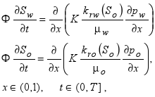(1)

where the unknowns are the pressures, p_w, p_o, and the saturations, S_w, S_o. The absolute permeability, K; the porosity, Φ, and the water and oil viscosities, μ_w, μ_o are constant parameters, whereas the relative permeabilities for oil and water, k_rw, k_ro, are functions of the oil saturation only.

We denote by S_or the residual oil saturation, by S_wc the connate water saturation and by p_a the atmospheric pressure. With this notation, the initial conditions are

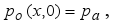	(2)
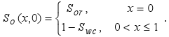	(3)

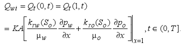
Boundary conditions are selected to reproduce the laboratory experiment as follows.

The inlet boundary condition is constant injection water rate and residual oil saturation,

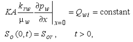(4)

where A denotes the cross-sectional area for the flow.

At outlet (x = 1), the boundary condition is imposed by the atmospheric pressure,

p_o(1,t) = p_a. (5)

Furthermore, we have the following three equations which relate the different variables.

Pressures in the oil and water phases are related by capillary pressure P_c as follows,

p_o - p_w = P_c(S_w). (6)

Also, oil and water saturations are connected by the condition,

S_o + S_w = 1. (7)

Finally, since the total flow rate Q_t (Q_t = Q_o + Q_w) is constant because the fluids are incompressible, we have,

(8)

A. The simplified model

As we stated in the introduction, the model described above will be simplified by imposing extra hypotheses.

First, to avoid the difficulty of dealing with discontinuous solutions we assume that the initial condition for S_o in (3) is a continuous approximation to the discontinuous initial function S_o(x,0).

The hypothesis that will allow us to deal with a simpler equation is that P_c(S_w) is constant. The simplification is carried out as follows: First, we add Eqs. (1) to obtain the system:

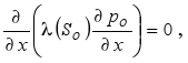	(9)
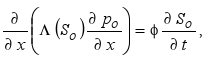	(10)

where

(11)

Equation (9) is the pressure equation.

To obtain the saturation equation we proceed as follows. From (8) and (9) is Q_wi / A, which is constant. Replacing this in (10) we obtain

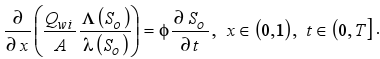(12)

The equation above is the saturation equation. Notice that a symmetric equation is obtained if we choose S_w instead of S_o: the functions that are increasing in one case are decreasing in the other.

Equation (12) is the usual conservation law equation,

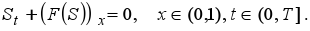(13)

In our case, 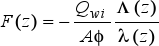. The function is the oil-fractional flow.

As we pointed out in the introduction we will deal with the saturation Eq. (12), thus we drop the subindex o.

Equation (13) is equivalently written as

(14)

where P = F'.

Now we consider Eq. (14) with initial condition

S(x,0) = f(x) x ∈ [0,1], (15)

where f is a given function.

It is well known that problem (14)-(15) does not have a solution unless stringent conditions are imposed. Also the solution might exist in a classical sense during an interval of time and then develop shocks or rarefaction.

The following is proposition 2.1.1 in the book by Serre (1999, page 26). It establishes the well posedness of (14)-(15) and guarantees a classical solution in an interval of time.

Proposition 1We assume that the function P ∈ C^∞(R) together with its derivative are bounded, and that f is of class C¹. We define T^* = +∞ if is increasing, and

(16)

otherwise. Then (14)-(15) possesses one and only one solution of class C¹in the band R×[0,T^*] and does not possess any solutions in any greater band than R×[0,T^*].

III. THE ESTIMATION PROBLEM

From now on, to highlight the dependency of S on the parameter P, we will denote S by S(P).

We assume that f is of class C¹ and monotonous.

We define the set of admissible parameters as

(17)

The map

P → S(P) (18)

maps the C^∞ function P into the C¹ function S.

Our aim is to estimate the function P(z) given measurements of the solution of the initial value problem (14)-(15).

The measurements, which are denoted by S^obs(t), are the values of the saturation at a recording point x^rec, for times in the interval [0,T], where T is a given time. Thus, for parameters in the set P, there is a classical solution on any interval [0,T].

The problem is to find P^* such that S(P^*)(x^rec,t) matches the values of S^obs(t), for t ∈ [0,T]. Specifically: find P^* such that

S(P^*)(x^rec,t) = S^obs(t), t ∈ [0,T]. (19)

Let Q be a subset of C¹([0,∞)). The parameter to-output-mapping

(20)

is continuous. This fact can be proved using the solution of (14)-(15) given by the method of characteristics.

The algorithm that we will use is also called a quasilinearization algorithm. It is based on the linearization of S as a function of P, about a particular function .

The linearization of S(P) about is:

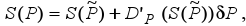(21)

where D'_P is the differential of S with respect to P.

Notice that we are differentiating with respect to the parameter P, which is a function. Therefore D'_P is a functional derivative, it is the Fréchet derivative (Ortega and Rheinboldt, 1970). We recall that the Fréchet derivative is a generalization of the differential of a function between Euclidean spaces and it behaves in an similar way.

A. The Fréchet derivative of S with respect to P

In the present subsection we describe how to compute the term D'_P(S())δP in Eq. (21) for a given . Specifically, the function D'_P(S())δP denotes the application of the operator D'_P to the function δP.

The procedure to calculate D'_P(S())δP involves the solution of an auxiliary differential equation followed by its multiplication by δP composed with S(). The mathematical details are cumbersome and will be presented in a suitable publication.

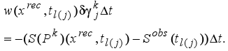
The starting point to compute D'_P(S())δP, for a given δP is to calculate the solution S of the conservation law (14), with initial condition (15) for P = . With the computed S we state the auxiliary equation on the function w:

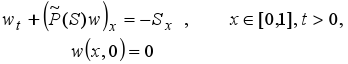(22)

Finally, for a given δP, with the calculated S and w we arrive at the desired formula, that is:

D'_P (S()) δP(x,t) = w(x,t) δP(S()(x,t)). (23)

Notice that Eq. (22) is linear.

Observation: the solution of (22) shows that the sign of w is equal to that of -S_x. Therefore the function w is always negative because S_x is positive. This observation is important for the implementation of the algorithm.

B. The quasilinearization algorithm

The algorithm is iterative, here we describe how each new iteration is updated from the previous one.

For a given the solution P^* of Eq. (19) can be written as P^* = + δP. Now, we linearize Eq. (19) using (21), at x = x^rec we obtain the following equation in the unknown δP:

D'_P (S()) δP = S^obs - S(). (24)

The above equation has a solution because S^obs - S() is in the range of D'_P (S()), see theorem 2.6 page 35 of Engl et al. (1996).

A least squares solution of Eq. (24) is a solution of the normal equation. That is, the solution of

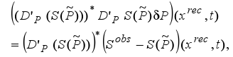(25)

where (D'_P)^* denotes the adjoint operator of D'_P considering the extension of the operator to the space L²([0,T]).

Using the observation at the end of the previous subsection it can be proved that S^obs(t) - S()(x^rec,t) is in the range of D'_P, therefore Eq. (25) has a solution.

IV. NUMERICAL IMPLEMENTATION OF THE ALGORITHM

In this section we describe the discretization to carry out the numerical implementation of the continuous algorithm.

The algorithm is iterative: given an initial guess P⁰, which is a value that belongs to the set of admissible parameters, we obtain the iterations P^k, k = 1,...; by correcting it with an appropriate δP as in (21).

We recall the basic steps of the algorithm.

1. Give an approximation of P^*,
2. Calculate an increment δP solving (25),
3.Update P as P_new = + δP.

Let t_j, j = 1,...,M; be the discrete times at which we make the observations. We assume that t_j are equally spaced, thus, we denote t_j - t_j-1 by Δt.

A. The discrete model of the parameter function P

First we approximate the function P to make it amenable to the calculations. Its approximation is given in terms of spline functions.

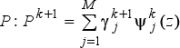
We seek functions P(z) of the form,

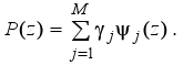(26)

To define ψ_j(z) we make a partition {z_j}, j=1,...,M; of the domain of P, such that z₁<z₂<... < z_M. The elements we choose are the first order ones:

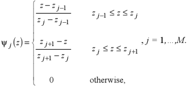(27)

B. Discretization of the normal equation

We give an initial guess of P(z):.

Next we specify the procedure for each iteration k≥0.

First we calculate S(P^k)(x^rec,t). Since P^k is a piecewise linear function, the solution of (14)-(15) can be calculated by solving the following (non-linear in most cases) equation on S(P^k)

(28)

where j is chosen to satisfy:

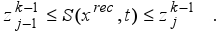(29)

Now, with S(P^k)(x^rec,t) computed above, we define a partition of the domain of P^k by points as follows

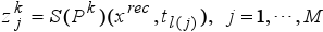(30)

where l(j) = j if f is non-increasing and l(j) = M - j + 1 if f is non-decreasing. We notice that in the algorithm the nodes z_j and, as a consequence, the functions ψ_j of Eq. (27) change at each iteration k, to remark it we denote the coefficients and the functions in (26) by and respectively.

Next, we express P^k and the unknown increment δP^k using the discretization of the previous subsection. Explicitly, the increment δP^k is

(31)

To determine , j=1,...,M; we solve (25) for S() = S(P^k) and δP = δP^k.

The computation of the discrete version of (25) requires tedious calculations, which are detailed in the Appendix and lead to the simple formula:

(32)

Solving for :

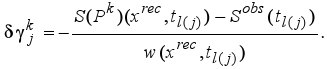(33)

By using (33) in (31) we compute δP^k and update P^k,

P^k+1 = P^k + δP^k (34)

The stopping criterion is that the residual

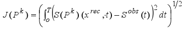(35)

must be small.

It can be proved that the sequence P^k converges monotonically to P^*.

C. Outline of the algorithm

1. Read , j = 1,..., M and the stopping criterion TOL.
2. Give an initial guess P⁰, set k = 0.
3. Solve the initial value problem (14)-(15) with P = P^k. Compute S(P^k)(x^rec,t).
4. Compute the residual J(P^k), Eq. (35).
5. If J(P^k) < TOL then P^k is the solution, STOP.
6. If not,

For j = 1,...,M

• Define .
• Compute .
• Compute w(x,t) solving the initial value problem (22) with P = P^k.
• Compute applying (33).
• Define .

end for.

• Update .
• k = k+1, go to 3.

V. NUMERICAL EXPERIMENTS

We illustrate the performance of the algorithm with two examples.

In the first one, the parameter P is on the set of admissible parameters ( increasing). The hypotheses of Proposition 1 are satisfied, thus a solution for every time exists. In the second one is not increasing therefore a classical solution of the direct model exists for intervals [0,T], with T < T^*.

In both examples we select the well known potential model (Lake, 1989) for relative permeabilities.

In the first one k_ro(S) = S and k_rw(S) = 0.2 (1 - S), thus the parameter to estimate is 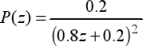. The initial condition is f(x) = 1 - x which is also decreasing.

Figure 1 shows snapshots of the saturation for t = 0.25, 0.5, 0.75, 1.0. In Fig. 2 we plot the 'true' parameter P, the initial guess P⁰ and the final estimate P^*. Convergence was achieved in 8 iterations. The residual was required to be smaller than 10^-7. The sampling times are t = k*0.05, k = 1,..., 20. The recording points are x^rec = 0.98 and x^rec = 0.3. An almost exact match to the 'true' function is obtained

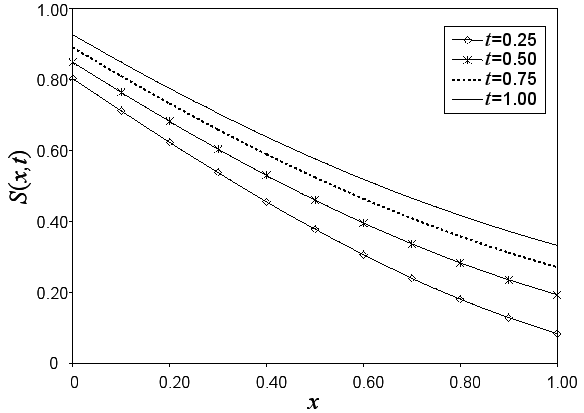
Figure 1: Saturation profiles

Figure 2: Estimation of the derivative of the fractional flow curve

In the second example the hypothesis of being increasing is not satisfied for every t. Despite, it is possible to estimate P on all its range using different positions of the receiver.

In this case k_ro(S) = S² and k_rw(S) = 0.2(1 - S)² thus the parameter P(z) is the function

(36)

and the initial condition is f(x) = x. Therefore, according to Proposition 1, the solution of (14)-(15) exists in the classical sense and is unique for t ∈ ⌊0, T^*), where T^* ≈ 0.14 which is 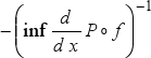, that infimum is attained approximately at z = 0.4.

Figure 3 depicts some characteristic curves for t ∈ [0,1]. We can observe that the characteristics intersect as we can expect for t > T^*. Figure 4 is a zoom of Fig. 3 up to t ≈ T^*.

Figure 3: Characteristic lines of the second example

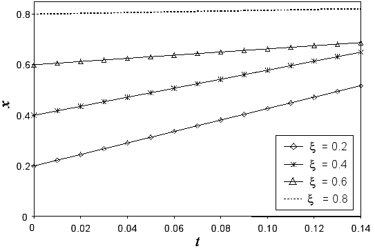
Figure 4: Characteristic lines for t ∈ [0,T^*]

Figure 5 shows snapshots of the saturation for various times for P(z) given by (36). Classical solutions exist only up to T^*, the saturation curves after T^* are entropy solutions, they were computed using the method of characteristics.

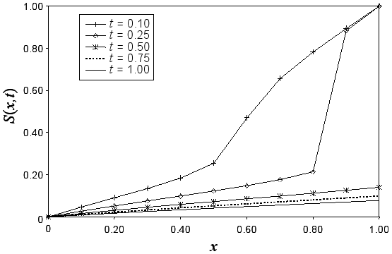
Figure 5: Saturation profiles for P(z) defined by (36)

Since the classical solution exists up to time T^* the range of S(x^rec,t), t ∈ [0,T^*] for a given x^rec is narrow: it does not cover the interval where the solution exists in the weaker sense (Fig. 5).

Despite the local behaviour of the estimation, placing receivers at different locations it is possible to estimate P on almost all the range of the saturation.

Figure 6 illustrates the previous claim, showing the estimation obtained for different positions of the receiver. Again, the residual was required to be smaller than 10^-7 and convergence is achieved in 8 to 12 iterations, depending on the location of the receiver.

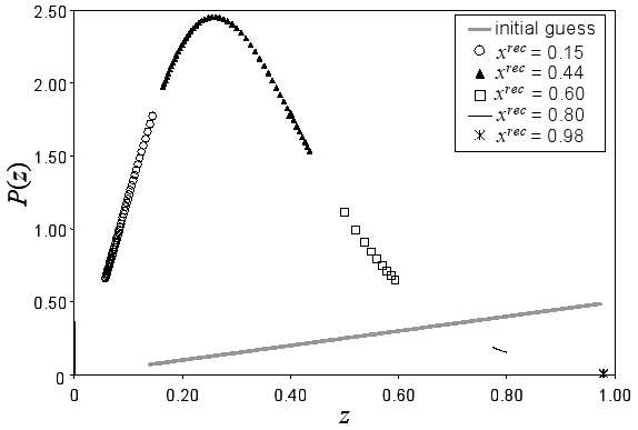
Figure 6: Estimation of P(z) using five receivers

The reason why it is possible to estimate different ranges of z depending on the position of the receiver x^rec lies in the equation for the characteristic lines passing through x^rec

x^rec = ξ + P(f(ξ))t. (37)

In conclusion, it is possible to estimate P on different ranges of its domain choosing the location of the recording points.

VI. CONCLUSIONS

An algorithm to solve an estimation problem in a non-linear differential equation is introduced. This algorithm is based on the least squares criterion in functional spaces and therefore an infinite dimensional estimation problem is solved. The sensitivity equation that is used to compute the Fréchet derivative is presented. The resulting algorithm has shown convergence in numerical tests, and because of its general theoretical formulation has the potential to be extended to solve more complex problems. This algorithm obtains the sought-after parameters without the imposition of a priori parametric models. Though the use of such models is currently the common practice among field engineers, different models yield different results and there is no objective criterion to choose among them. Thus the result yielded by the different parametric models can be compared to those of our algorithm, so as to select the best fitting model.

VII. APPENDIX

We show the steps that lead to Eq. (32) starting from its continuous version (25) and using the discrete versions of P and S(P).

We denote by Ψ the subspace of generated by the set of functions . From Eq. (26) P^k ∈ Ψ. From Eq. (28) S(P^k)(x^rec,·) ∈ L²([0,T]), therefore, D'_P(S(P))δP(x^rec,·) ∈ L²([0,T]), specifically,

D'P:Ψ→L2([0,T]),	(38)
δP(z)→D'P(S(P))δP(xrec,t)

as a consequence,

(D'_P)^*:L²([0,T])→Ψ. (39)

To compute the coefficients of δP we proceed as usual. We calculate the scalar product of (25) with an element of the basis of Ψ.

The computation of the left hand side, for j = 1,...,M; results in the following equation

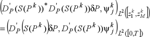(40)

Using Eq. (23) to replace D'_P(S(P^k)) in the above equation and writing explicitly the scalar product in L²([0,T]), Eq. (40) equals to

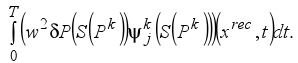(41)

Discretizing Eq. (41) in t, using the definition of and that of in Eq. (30), we obtain the chain of equalities:

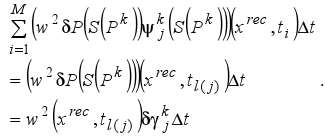(42)

Similarly, the right hand side of (25) is,

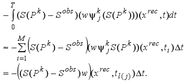(43)

REFERENCES
1. Aziz, K. and A. Setttari, Petroleum Reservoir Simulation, Elsevier Applied Science Publishers, Great Britain (1985).         [ Links ]
2. Bech, N., D. Olsen and C.M. Nielsen, "Determination of Oil/Water Saturation Functions of Chalk Core Plugs From Two-Phase Flow Experiments", Society of Petroleum Engineers Reservoir Evaluation and Engineering, 3, 50-59 (2000).         [ Links ]
3. Chardaire-Riviere, C., G. Chavent, J. Jaffre, J. Liu and B.J. Bourbiaux, "Simultaneous Estimation of Relative Permeabilities and Capillary Pressure", Society of Petroleum Engineers Formation Evaluation, 7, 283-289 (1992).         [ Links ]
4. Engl, H., M. Hanke and A. Neubauer. Regularization of Inverse Problems Kluwer Academic Publishers, Dordretcht (1996).         [ Links ]
5. Fernández-Berdaguer, E.M., "Parameter estimation in acoustic media using the adjoint method", SIAM Journal on Control and Optimization, 4, 1315-1330 (1998).         [ Links ]
6. Fernández-Berdaguer, E.M., P. Gauzellino and J.E. Santos, "An Algorithm for Parameter Estimation in Acoustic Media Practical Issues", Latin American Applied Research, 25, 161-168 (1995).         [ Links ]
7. Fernández-Berdaguer, E.M., J.E. Santos and D. Sheen, "An Iterative Procedure for Estimation of Variable Coefficients in a Hyperbolic System", Applied Mathematics and Computation, 76, 213-250 (1996).         [ Links ]
8. Kruger, H., A. Grimstad and T. Mannseth, "Adaptive multiscale estimation of a spatially dependent diffusion function within porous media flow", Inverse Problems in Engineering, 11, 341-358 (2003).         [ Links ]
9. Lake, L.W., Fundamentals of Enhanced Oil Recovery, Prentice Hall, New Jersey (1989).         [ Links ]
10. Mejía, G.M., K.K. Mohanty and A.T. Watson, "Use of In Situ Saturation Data in Estimation of Two-Phase Functions in Porous Media", Journal of Petroleum Science and Engineering, 12, 233-245 (1995).         [ Links ]
11. Ortega, J.M. and W. Rheinboldt, Iterative solution of nonlinear equations in several variables, Academic Press, New York (1970).         [ Links ]
12. Savioli, G.B. and M.S. Bidner, "Comparison of Optimization Techniques for Automatic History Matching", Journal of Petroleum Science and Engineering, 12, 25-35 (1994).         [ Links ]
13. Savioli, G.B. and M.S. Bidner, "Interpretación Automática de Ensayos de Flujo Bifásico en Medios Porosos", Revista Internacional de Métodos Numéricos para Cálculo y Diseño en Ingeniería, 11, 131-150 (1995).         [ Links ]
14. Serre, D., Systems of Conservation Laws, Cambridge University Press (1999).         [ Links ]
15. Tarantola, A., Inverse Problem Theory - Methods of data fitting and model parameter estimation, Elsevier (1987).         [ Links ]
16. Valestrand, R., A. Grimstad, K. Kolltveit, J. Nordtvedt, J. Phany and T. Watson, "Extension of Methodology for the Determination of Two-Phase Porous Media Property Functions", Inverse Problems in Engng., 11, 289-307 (2003).         [ Links ]

Received: May 22, 2006.
Accepted: December 18, 2006.
Recommended by Subject Editor Orlando Alfano.