Analysis of heat and mass transfer in a mixed convective diffusion flame attached to a vertical fuel surface

A. J. Bula¹ and M. M. Rahman²

¹ Departamento de Ingeniería Mecánica, Universidad del Norte, Kilómetro 5 Antigua Vía Puerto Colombia, Barranquilla, Colombia. abula@uninorte.edu.co
² Mechanical Engineering Department, University of South Florida, 4202 E Fowler Av, Tampa, FL, 33620, USA
rahman@eng.usf.edu

Abstract — Analysis of heat and mass transfer in a burning vertical surface exposed to a fluid flow parallel to the surface is presented. The combustion process considered is steady and the burning surface is in equilibrium vaporization. A fast gas phase reaction is assumed to occur between the fuel and the oxidizer. The flame sheet approximation is used to describe the reacting flow. The governing equations describing the conservation of mass, momentum, energy, and species concentrations were solved numerically along with appropriate boundary conditions. Schvab-Zeldovich variables were used to eliminate the mass and energy generation terms from the governing equations. Calculations were done for two different fuels and for a range of Reynolds number. Computed results included the distributions of velocity components, enthalpy, and concentration of fuel, oxidizer, products, and inert gas, and the position of the flame sheet.

Keywords — Diffusion Flame; Conjugate Heat Transfer; Heat and Mass Transfer.

I. INTRODUCTION

Diffusion flames are observed during the combustion of a solid, liquid, or gaseous fuel. Some common examples include fires, furnaces, and burners. Many of these combustion processes occur under the combined influence of a vertical buoyant flow and an external forced flow. The analysis of such a mixed convective flow is the objective of the present investigation.

The laminar natural convective burning of a vertical fuel surface was first addressed by Spalding (1954). After making several simplifying assumptions, a similarity solution was obtained for the boundary layer flow on a flat surface. Williams (1985) introduced a mathematical transformation, known as the Schvab-Zeldovich transformation, to simplify the governing equations. Shih and Pagni (1978) described a laminar, free and forced, mixed-mode diffusion flame adjacent to a vertically burning fuel slab using Schvab-Zeldovich variables, boundary layer and local similarity approximations. The solution presented flame position, concentrations, velocity profiles and surface fluxes, and showed that the flow characteristics were more complicated than superposition of two limiting flame cases. Kinoshita and Pagni (1980) performed a numerical analysis of a steady, laminar, two-dimensional, non-radiative boundary layer. Based on the results, explicit functional fits to numerical flame heights were obtained for free and mixed-mode flows. The comparison with theoretical results indicated quantitative agreement. Liu et al. (1981) solved the two dimensional laminar thermo-buoyant flow diffusion flame with the gaseous fuel injected uniformly through the vertical surface. Fernandez-Pello and Pagni (1983) performed an analysis for mixed, forced, and free convective combustion on a vertical fuel surface which made use of the laminar boundary layer approximation to describe the gas flow and the flame sheet approximation to describe the gas phase reaction. They used a parameter as a function of Reynolds and Grashof number to develop a solution that is uniformly valid over the entire range of mixed flow intensities. Kodama et al. (1987) investigated the process of extinction and stabilization of a diffusion flame on a flat combustible surface for oxidizing gas flow parallel to the fuel surface. Theoretical results were validated using a simplified experimental approach. Di Blasi (1994) developed a two dimensional, unsteady model of the degradation of porous cellulosic fuels to volatiles and chars to simulate downward flame spread. Ray and Wichman (1998) numerically investigated a diffusion flame using a model heat loss profile. The radiative intensity, width, and location of the heat loss profile were parametrically varied to assess the sensitivity of the flame to heat losses. The emphasis was placed in the extinction of the flame due to increased heat losses. Costa (1998) studied the effects of differential diffusion on unsteady one-dimensional diffusion flame. Bula and Rahman (1998) analyzed a diffusion flame adjacent to a burning vertical surface exposed to a horizontal fluid flow parallel to the surface. Calculations were done for two different fuels and for a variety of Reynolds numbers. The computed results included the distributions of velocity components, enthalpy, and concentration of fuel, oxidizer, products, and inert gas in the entire boundary layer region. Ramadan (2003) studied the effect of the Damkohler number and non-unity Lewis number on a two-dimensional, steady, laminar diffusion flame anchored by a dividing plate in a rectangular channel. The results showed that an increase in the Da causes the flame to exist closer to the trailing edge of the divider and to increase the reactivity. A non-unity Lewis number creates a non-symmetrical flame by forcing the flame to exist on the fuel side. Nayagam and Williams (2002) employed activation-energy asymptotics to explore effects of the Lewis number, the ratio of thermal to fuel diffusivity, in a one-dimensional model of steady motion of edges of reaction sheets. The results show that increasing the Lewis number increases the propagation velocity at large Damkohler numbers and decreases it at small Damkohler numbers. Advancing-edge and retreating-edge solutions are shown to exist simultaneously, at the same Damkohler number, if the Lewis number is sufficiently large. Liu et al. (2005) presented the soot inception processes in nonpremixed flames in a spherical flame stabilized by a spherical porous burner to understand the effects of flame structure (stoichiometric mixture fraction) and hydrodynamics (flow direction). They presented three distinct reaction zones. The analysis yields a solution giving the flame response to the variations of the soot formation and consumption reaction rates, the mass-flow rate issued from the burner, the Lewis numbers, and the inert distribution.

From the above literature review, it is noticed that the Lewis number equal to 1 to simplify the analysis has been changed, considering the appropriate Lewis number at the combustion area. In the present investigation a two-dimensional boundary layer flow adjacent to a vertical pyrolyzing wall is analyzed when buoyancy-driven reacting flow and transport is superimposed on a forced flow in the vertical direction, and Lewis number different from one is used to calculate different parameters involved in the problem. Equations governing the conservation of mass, momentum, energy, and species concentration were solved numerically to predict velocity, temperature, and concentration distributions across the boundary layer and the variation of heat and mass transfer rate over the plate. A parametric analysis is performed to study the effects of Re, Sc, and Le. The combustion characteristics of two different materials: polymethylmethacrylate (PMMA) and heptane were simulated in order to explore the effects of Schmidt number.

II MATHEMATICAL MODEL

A laminar, steady state, two dimensional boundary layer flow, and the diffusion flame adjacent to a pyrolyzing fuel slab, as shown in Fig. 1 is considered. It is assumed that the combustion process is steady and the burning surface is in equilibrium vaporization, i.e., the activation energy in the surface pyrolysis is sufficiently large that the variation in the surface mass flux, required by the boundary layer, can be accommodated with negligible change in surface temperature. In addition, a fast gas phase reaction is assumed to occur between the fluid and the oxidizer. Since the characteristic time of gas phase reaction is much longer than the chemical kinetics time scale the combustion zone is thin and the reactants (fuel and oxidizer) do not coexist and are at either side of the flame sheet. The equations describing the conservation of mass, momentum, energy, and species concentration can be written as:

	(1)
	(2)
	(3)
	(4)

where h and C_p of the mixture can be defined as:

(5)

Figure 1. Schematic of geometry considered

In Eqs. (4) and (5), the subscript 'i' refers to the species under consideration. Even though the chemical reactions occurring in a combustion process are fairly complicated, in a very simplified form, a mathematical model can be developed by considering only four species, namely, fuel, oxidizer, products, and inert gases. In Eq. (3), the viscous dissipation and pressure work terms are neglected because they are of lower order of magnitude compared to convection terms in a low speed gas flow. An equation of state is required for the fluid. Considering the fluid to be an ideal gas with no change in the average molecular weight leads to:

(6)

The chemical reaction can be represented as:

(7)

The molecular coefficients of Eq. (7) can be calculated from a chemical balance. The species mass production rate is related to the energy generation rate by:

(8)

To complete the set to be solved, Eqs. (1-4) are subject to the following boundary conditions:

(9)

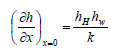
The remaining boundary conditions at x = 0 are obtained from pyrolysis at the wall. From energy balance:

(10)

From mass balance:

	(11)
	(12)
	(13)

It may be noted that both mass and energy balance have to be satisfied at the wall. The rate of heat transfer to the wall determines the rate of pyrolysis, which in turn controls the blowing velocity at the wall. The volumetric energy generation rate q''' and the volumetric rate of species generation m_i''', are complicated functions of at least temperature and species mass fraction. Even in the presence of a single step, second-order Arrhenius expression, uncertainties in the values of the expression remain. Nevertheless, in order to solve this problem, the mass and energy generation terms are removed from the equations through the use of the Schvab-Zeldovich variables (Shih, 1984). The major assumption associated with this formulation is that the mass fluxes of reactants are in stoichiometric proportion at the flame position. For a laminar diffusion flame, this imposes the condition that the reactants do not coexist. The advantage is that only one species equation needs to be solved in any part of the computational domain. These two variables can be defined as:

(14)

With these new variables, Eqs. (3) and (4) can be written as:

	(15)
	(16)

The second term in the right-hand side of Eq. (15) drops out in the fuel region (next to the wall), but it cannot be neglected in the oxidant region. In order to avoid this inconvenience, a new Schvab-Zeldovich variable was defined, but using quantities relevant to the fuel.

(17)

With this new variable, Eq. (3) becomes

(18)

In this equation, the second term on the right-hand side drops out in the oxidant region, but cannot be neglected in the fuel region. It is convenient to define the following nondimensional parameters at this point:

(19)

The value of is calculated using the flame location determined from , which depends only on the properties of the pyrolyzing fuel and the ambient medium. The position of the flame can be obtained from (Fernandez-Pello and Pagni, 1983)

(20)

The governing Eqs. (1-2,15,16,18), can be expressed in terms of the dimensionless variables as:

	(21)
	(22)

where G is defined as follows:

for :

(23)

and

for :

(24)

where:

	(25)
	(26)
	(27)
	(28)

where:

(29)

The boundary conditions in terms of dimensionless variables are:

At X = 0:

	(30)
	(31)

where B is defined as:

	(32)
	(33)

At X → ∞

(34)

At Y = 0

(35)

At X =

(36)

From Eq. (31), the mass transfer number can be expressed as:

(37)

It should be noted that if Eq. (27) is solved for the fuel region and Eq. (28) is solved for the oxidant region, then the second term on the right-hand side of each equation drops out, and the two equations are identical. Therefore, these equations can be expressed as a single equation and can be solved with boundary conditions relevant to each region. However, to evaluate the buoyancy term and recover the values for enthalpy and density, Eq. (14) and Eq. (17) must be used according to the region under consideration (fuel or oxidizer). We will now refer to the energy equation only with :

(38)

The enthalpy and the mass concentration for oxidant and fuel can be obtained from the following equations:

for :

(39)

for :

(40)

To recover the concentration of oxidant, fuel, inert gas (nitrogen), and products the following equations are required.

If :

(41)

If :

(42)

Since nitrogen is an inert gas, its nondimensionalized mass fraction also satisfies the J_β transport equation if m_nw is considered constant. Consequently,

(43)

where

(44)

Once m_n, m_o, m_f are calculated, the assumption that fuel and oxidant do not coexist yields:

If :

(45)

If :

(46)

The ratio included in the definition of the mass transfer number B, Eq. (37), depends on the properties of the medium of diffusion and the diffusing substance.

Equations (26) and (38) are similar except that one depends on Sc and the other depends on Pr. These two parameters can be related by Lewis number (Le = Pr / Sc). Depending on which of these is larger, the thickness of the zone of influence will be larger. As the limit for and J_β are equal (0 - 1), the derivatives can be equal only when Le = 1; and as the thickness of the influence zone increases, the first derivative decreases and vice versa. For Le < 1, the thickness of each influence zone is shown in Fig. 2. At a location "a", the influence zone of J_ζ is larger than the zone of J_β, and is less than . This leads to a ratio less than one, which is in accordance with the Lewis number. The same procedure can be applied for Le > 1 and Le = 1. This relation between the ratio of the first derivatives with the Lewis number can be used to obtain an expression for the mass transfer number depending only on characteristics of the fuel, oxidant, and the values of the concentration of the reactants at the wall and at the free stream.

Figure 2. Development of and J_β for Le < 1.

The derivatives of J_β and can be obtained as:

	(47)
	(48)

From mass balance expressed as a function of the mass transfer coefficient, the second factor on the right-hand side of Eq. (47) can be expressed as:

(49)

From energy balance expressed as a function of the convective heat transfer coefficient, the second factor on the right-hand side of Eq. (48) can be expressed as:

(50)

In order to obtain a relation between the heat and mass transfer coefficients, the Colburn 's analogy (Cheremisinoff, 1986) is used. This correlation is expressed as:

(51)

Substituting Eqs. (49) and (50) into Eqs. (47) and (48), and using Eq. (51), the ratio can be expressed as:

(52)

To obtain the final equation for the mass transfer number, the expression obtained for the ratio of the first derivatives as shown in Eq. (52) is substituted into Eq. (37). After some simplifications, the following equation is obtained.

(52)

From Eq. (52) it can be observed that the ratio is a function of the fuel concentration at the wall, which is also unknown. Therefore, the solution requires a trial and error procedure. The correction factor C _f can be obtained from the physics of the problem, i.e., Eq. (31) must be satisfied. First, Lewis number equal to one is assumed. This makes the ratio expressed in Eq. (52) to become 1. Therefore, the mass transfer number B, can be calculated from Eq. (37). Substituting B in Eq. (32) allows the calculation of the fuel concentration at the wall. This value is then used in Eq. (53) to get the correction factor. As soon as C_f is obtained, the fuel concentration and the mass transfer number can be calculated for the real Lewis number. Using the fuel concentration at the wall (starting with the solution for Le = 1), the mass transfer number is calculated from Eq. (32) and Eq. (53). Iterations are continued until the values of B returned from both equations are equal.

III. RESULTS AND DISCUSSION

The mathematical model developed in the last section was solved using a control volume based finite-difference method. In each cell, the velocity components were stored at downstream boundaries, whereas, pressure, enthalpy, and concentrations were stored at the center of the cell. In order to keep the relative contribution of convection and diffusion to a cell from its neighbors in terms of cell Peclet number, the hybrid difference scheme demonstrated by Patankar (1980) was used. The discretized equations were solved using the SIMPLEST algorithm (Spalding, 1980). Computation was done in an iterative fashion starting with a guessed pressure field. The momentum equations were solved to obtain the velocity components. The continuity equation was modified to a pressure correction equation (Patankar, 1980) that updated the pressure field. In the present model, the buoyancy force couples the energy and momentum equations. In addition, energy and species transport equations are coupled to each other via nondimensional variables and J_β. Therefore, all equatios had to be solved simultaneously. The momentum and continuity equations were solved slab-by-slab using a slabwise linear solver. The solution marched on the z-direction and solved for each slab at a particular z position. This procedure was repeated for a number of sweeps from the lowest to the highest z position. The energy and concentration equations, in their dimensionless form, were solved simultaneously for the entire computational domain.

The iterative solution was continued until the sum of the residuals for all computational cells became negligible (less than 0.001%) and the velocity components and other scalar variables did not have any significant change (less than 0.0001 %) between iterations. Numerical simulations were done for the burning of a vertical wall of PMMA (Polymethylmethacrylate) and the combustion of heptane injected from a porous vertical wall (Perry, 1984). A typical grid independence analysis is shown in Fig. 3. It can be noticed that the solution becomes grid independent when 90 divisions are used in the x-direction. Values of J_β remain identical when number of grids in the x-direction is increased to 120. It was found that 60 divisions in the y-direction are adequate to produce grid independent numerical solution over the entire computational domain. Despite having an independent solution with the grid size mentioned before, the number of divisions in the x-direction and y-direction were increased to 120 and 80 respectively in order to obtain a very smooth variation of solution over the computation domain.

Figure 3. Grid analysis

In order to validate the model presented in this paper, the flame position was compared with the results given by Fernandez-Pello and Pagni (1983). This comparison was carried out using Le=1, and pyrolyzed PMMA as the fuel and it is presented in Fig. 4. Computed results are presented for Re = 250, 500, and 19500. Also shown are natural and forced convection limits from the analytical solution of Fernandez-Pello and Pagni (1983). It may be noted that flame sheets for mixed convection at all Reynolds numbers are bounded by natural and forced convection limits. At Re = 250, the flame position above 0.08 m matches the solution of Fernandez-Pello and Pagni (1983) for natural convection. At this Reynolds number, the forced flow velocity is small, and therefore its effects are limited to a small region near the leading edge. The flow is driven primarily by buoyancy induced motion. The flame position corresponding to Re = 19500 is not too far from the analytical solution for the forced convection limit. It may be noted that, while in the analytical solution, the buoyancy effects can be terminated by assuming Re → ∞, in a practical combustion process, the effects of buoyancy can not be neglected entirely because of large temperature difference between the flame sheet and the ambient. Moreover, at higher Reynolds number the flow becomes turbulent which was not accounted for in the mathematical model. Considering these limitations, the comparison between the analytical solution of Fernandez-Pello and Pagni (1983) and the present numerical solution is quite satisfactory.

Figure 4. Flame position for Le = 1 and different Reynolds number

Figure 5 presents the flame position for different values of Lewis number and Re = 250. It can be seen that when Le = 1 (Pr = Sc = 0.7), the shape of the flame matches nicely with the analytical solution from (Fernandez-Pello and Pagni, 1983). But when the parameters are changed to Le = 1 (Pr = Sc = 1.7), the curve gets closer to the one predicted for Le = 0.4 (Pr = 0.7, Sc = 1.7). This shows that Schmidt number is the primary factor that determines the position of the flame and must be accounted for during the simulation of a combustion process. In Fig. 5 it can be observed that the flame position stands further away from the burning fuel slab when Le = 1 (Pr = Sc = 0.7) is used. Even though the assumption of Le = 1 has been made in several past analytical as well as numerical work, the error introduced with this assumption appears to be fairly large. The other point to be considered is that the approximation of Le = 1 is hardly obtainable when burning a pyrolyzed fuel. The lightest fuel considered would be Methane (CH₄), which has Sc = 0.84, giving Le = 0.83. As the molecular weight of the fuel increases, the Schmidt number increases too, for example, Heptane (C₇H₁₆), with Sc = 1.22 and Le = 0.57. For an n-Octane fuel, Schmidt number is approximately equal to 2.62 and this results in Le = 0.26. Therefore, Le = 1, is never present in a real diffusion flame. Therefore, it will be always advisable to use the real Lewis number in the analysis of a combustion process.

Figure 5. Flame position for Re = 250 and different Lewis number

The present analysis was done for two different materials: Polymethylmethacrylate (PMMA), with Le = 0.4; and heptane, with Le = 0.56. The Reynolds number used for both was 250. The mass transfer number and the fuel concentration at the wall were calculated for both materials. The values obtained were B = 0.95239 and m_fw = 0.42645 for PMMA, and B = 1.237 and m_fw = 0.524 for heptane. For the case of PMMA the flame position was located at J_βfl = 0.3041 and for heptane it was situated atJ_βfl = 0.1899. It is observed that for Le = 0.56 the flame sheet is located farther away from the wall than for Le = 0.4. This result was expected because the value of J_βfl for heptane is smaller compared to the value for PMMA. It can be noticed in Fig. 6 that as Reynolds number increases, the flame sheet (the plane where the reaction takes place), moves closer to the pyrolyzing wall. This happens because, as the forced flow velocity increases, it pushes the flame sheet against the wall.

Figure 6. Flame position for Le = 0.4 and different Reynolds number

On the other hand, Fig. 7 shows that the increment of the Reynolds number does not have any effect on the concentration of species at the wall, flame sheet, or ambient. This can be explained by the fact that none of the boundary conditions for oxidant, fuel, inert gases, or product are changed. At the flame sheet both fuel and oxidant reaches zero concentration due to complete combustion. The concentration of the products is determined by the chemical reaction and therefore not affected by the Reynolds number.

Figure 7. Concentration variation along the X axis at Y = 0.8 for Le = 0.4 and different Reynolds number

In Fig. 8 can be seen that the effects of Reynolds number on the enthalpy and density of the mixture are similar to that observed for concentration. This figure shows that the maximum enthalpy and minimum density are located at the flame sheet. This is in line with the physics of the problem. The chemical reaction takes place at the flame sheet liberating the maximum energy and reaching the maximum enthalpy. At the same place, the density reaches its minimum value. It is interesting to note, that the Reynolds number does not have any influence on the maximum dimensionless enthalpy reached by the reaction, in all cases analyzed this turned out to be 4.93. This is expected because of the rate of energy generation that controls the flame sheet temperature is determined by chemical kinetics.

Figure 8. Enthalpy and density variation along the X axis at Y = 0.8 for Le = 0.4 and different Reynolds number

The magnitude of enthalpy obtained in the solution is very close to the value reported by Kodama et al. (1987) for the combustion of PMMA. The minimum value for density was 0.14; equivalent to 0.165 kg/m³, which is consistent with the tabulated value for air at the same temperature, 0.168 kg/m³ (Kays and Crawford, 1993)

Figure 9 shows the distribution of velocity components across the boundary layer. It can be noticed that U velocity has a magnitude much smaller than V velocity, where U and V are the components of the velocity in the x, and y directions, respectively. This is consistent with the boundary layer approximation used for the formulation of the problem. V becomes maximum at the flame sheet, while U becomes minimum at the same location. The maximum U velocity is reached at the edge of the boundary layer. The local Grashof number at the flame position turned out to be 2.21x10⁶, which is within the range of the laminar buoyant flow assumed for the simulation (Gebhart et al., 1988). It can be noticed in Fig. 9 that the U velocity changes significantly with Reynolds number while the maximum value of the V velocity in the nondimensional form reduces as the Reynolds number increases. With the increase of Reynolds number, the values for V gets closer to w_∞, this is expected because the forced flow gets stronger while the natural flow remains constant. A larger magnitude of velocity near the flame sheet is due to larger temperature and smaller density in that region.

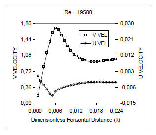
Figure 9. Velocity variation along the X at Y = 0.8 axis for Le = 0.4 and different Reynolds number

Figure 10 compares the enthalpy and density variation for the two fuels considered for this analysis. For both cases the maximum enthalpy is obtained at the flame sheet. It is important to note that the maximum value of the enthalpy in the non-dimensional form is reached by the heptane, but the corresponding dimensional value shows that the enthalpy of the PMMA is higher (2152 kJ/kg), compared to 540 kJ/kg for heptane. This is due to the higher value of the heat of reaction for the PMMA-air combination, which is 13.57x10³kJ/kg. The heat of reaction for the heptane-air combination is 3.03x10³kJ/kg. The flame temperatures are 2092 K for PMMA-air and 748 K for heptane-air. The minimum values of density are obtained at the flame sheet; in the non-dimensional form it is 0.14 for PMMA and 0.44 for heptane. In the dimensional form, these values are 0.165 kg/m³ and 0.49 kg/m³. These results are in good agreement with the ideal gas assumption.

Figure 10. Enthalpy and density variation along the X axis at Y = 0.8 for Re = 250 and different Lewis number

The velocity distributions for the two fuels are compared in Fig. 11. The velocities for PMMA are somewhat higher than heptane because of larger flame temperature. Figure 12 presents the concentration variation; it is seen that the variation of products and inert gases change when the concentration of the fuel at the wall is changed. For heptane, the concentration of products is higher than PMMA.

Figure 11. Velocity variation along the X axis at Y = 0.8 for Re = 250 and different Lewis number

Figure 12. Concentration variation along the X axis at Y = 0.8 for Re = 250 and different Lewis number

Figure 13 compares the results obtained with the present model to the experimental data of Kodama et al (1987) for the burning of PMMA in air. It is observed that the numerical prediction of flame position is quite accurate. The maximum deviation is only about 9%. The maximum thickness of the boundary layer recorded in their experiment was 0.75 cm, while the one obtained in the simulation was 0.76 cm. The maximum velocity measured experimentally was 0.65 m/s compared to 0.59 m/s obtained numerically. The maximum temperature showed reasonably good agreement as well; 2200 K experimentally, while 2100 K from numerical prediction.

Figure 13. Comparison between present numerical simulation and experimental data, Kodama et al (1987)

IV. CONCLUSIONS

The effects of different parameters have been simulated for a laminar diffusion flame under aiding mixed convection. It has been found that Reynolds number has a remarkable effect on the flame position and the size of the boundary layer. When the Reynolds number is increased, the flame sheet moves closer to the wall, and the maximum value of the V velocity is reduced. The concentration values at the flame sheet were not affected by the Reynolds number. The maximum enthalpy and minimum density always occurred at the flame sheet. The mass transfer number B, plays an important role. As it increases, the concentration of fuel at the wall and the concentration of products at the flame sheet increases. The flame moves away from the wall when B increases. The mass transfer number was found proportional to Le^2/3. Since the Prandtl number for air remains approximately constant, the variation of Lewis number essentially represents the effects of the variation of Schmidt number. For heptane, the rate of mass transfer is higher, and the maximum enthalpy reached by the reaction is 6 times the enthalpy at the wall. For PMMA this value was 4.92.

In order to improve the model, the radiation heat transfer process should be included due to the high temperature attained at the reaction zone. The addition of this term is expected to increase the amount of fuel generated by the pyrolizing wall.

NOMENCLATURE
B Mass transfer number
C_p Specific heat at constant pressure [kJ / kg K]
C_f Correction factor included in Eqs. (51-53)
D Binary mass diffusion coefficient [m²/2]
D_c Dimensionless heat of combustion, defined by Eq.(25)
g Acceleration due to gravity [m²/s]
G Buoyant force due to temperature and concentration, given by Eqs. (25) and (26)
h Specific enthalpy [kJ / kg]
h_Dp Mass transfer coefficient [kg/s m²]
h_Hp Heat transfer coefficient [W/ m² K]
H Height of the plate ( in the y-direction ) [m]
J Normalized Schvab-Zeldovich variable
k Thermal conductivity [W / m.K]
L Height of the plate [m]
Le Lewis number (Pr / Sc or D/αα)
L_v Latent heat of vaporization [kJ / kg]
Mass flux [kg/m²s]
m_i Species masss fraction [kg species/ kg mixture]
m_i''' Volumetric species generation rate, [ kg / m³s]
M Molecular weight (kg / kmol)
NX Number of grids in the x-direction
NY Number of grids in the y-direction
n_i Stoichiometric coefficient
Pr Prandtl number (v/α)
'' Heat flux at the solid fuel surface [W / m²]
''' Volumetric heat generation rate [W / m³]
Q Heat of combustion [kJ / kg of oxidizer ]
r Mass consumption number defined by Eq.(35)
R Dimensionless density (ρ/ρ_∞)
Re Reynolds number (υ_∞L/v)
Sc Schdmidt number (v/D)
T Temperature [K]
u Velocity component in the x-direction [m / s]
U Dimensionless velocity in X-direction, u/υ_∞
υ Velocity component in the y-direction [m / s]
V Dimensionless velocity Y-direction, υ/υ_∞
x Normal coordinate [m]
X Dimensionless normal coordinate, x / L
y Vertical coordinate [m]
Y Dimensionless vertical coordinate, y / L
Greek symbols
α Thermal diffusivity [m²/ s]
β Schvab-Zeldovich variable for species
μ Viscosity [kg / m s]
v Kinematic viscosity [m²/ s]
ρ Density [kg / m³]
ζ Schvab-Zeldovich variable for energy
Subscripts
f fuel
fl flame sheet
i species
n nitrogen (or inert)
o oxidant
p products
t transferred
w wall
β concentration dependent
ζ temperature dependent
∞ free stream condition
Superscripts
' reactants side ( stoichiometric )
'' products side ( stoichiometric )

REFERENCES
1. Bula, A.J. and M.M. Rahman, "Mixed convective burning of a vertical fuel surface in the presence of a horizontal cross flow", Numerical Heat Transfer; Part A, 34, 399-419 (1998).         [ Links ]
2. Cheremisinoff, N.P., Handbook of Heat and Mass Transfer, 1, Gulf, Houston (1986).         [ Links ]
3. Costa, F.S., "Effects of Differential Diffusion on Unsteady Diffusion Flames", International Communications of Heat and Mass Transfer, 25, 237-244 (1998).         [ Links ]
4. Di Blasi, C., "Processes of Flames Spreading over the Surface of Charring Fuels: Effects of the Solid Thickness", Combustion and Flame, 97, 225-239 (1994).         [ Links ]
5. Fernandez-Pello, A.C. and P.J. Pagni, "Mixed Convective Burning of a vertical fuel surface", ASME -JSME Thermal Engineering Joint Conference Proceedings, 4, 295-301 (1983).         [ Links ]
6. Gebhart, B., Y. Jaluria, R.L. Mahajan and B. Sammakia, Buoyancy Induced Flows and Transport, Hemisphere, Washington D.C., 265-347 (1988).         [ Links ]
7. Kays, W.M. and M.E. Crawford, Convective Heat and Mass Transfer, 3rd ed., McGraw-Hill, N.Y., 480-590 (1993).         [ Links ]
8. Kinoshita, C.M. and P.J. Pagni, "Laminar Wake Flame Heights", Journal of Heat Transfer, 102, 104-109 (1980).         [ Links ]
9. Kodama, H., K. Miyasaka and A.C. Fernandez-Pello, "Extinction and Stabilization of a Diffusion Flame on a Flat Combustible Surface with Emphasis on Thermal Controlling Mechanisms", Combustion Science and Technology, 54, 37-50 (1987).         [ Links ]
10. Liu, K.V., J.R. Lloyd and K.T. Yang, "An investigation of a Laminar Diffusion Flame Adjacent to a Vertical Flat Plate Burner", International Journal of Heat and Mass Transfer, 24, 724-730 (1981).         [ Links ]
11. Liu, S., B.H. Chao and R.L. Axelbaum, "A theoretical study on soot inception in spherical burner-stabilized diffusion flames", Combustion and Flame, 140, 1-23 (2005).         [ Links ]
12. Nayagam, V. and F.A. Williams, "Lewis-number effects on edge-flame propagation", Journal of Fluid Mechanics, 458, 219-228 (2002).         [ Links ]
13. Patankar, S.V., Numerical Heat Transfer and Fluid Flow, Hemisphere, Washington D.C. (1980).         [ Links ]
14. Perry, R. H., Chemical Engineers Handbook, McGraw-Hill, N.Y., 2129-2205 (1984).         [ Links ]
15. Ramadan, B., "Effect of Damkohler number and non-unity Lewis number on a laminar diffusion flame", ASME/JSME Joint Fluids Engineering Conference, 2C, 2117-2124 (2003).         [ Links ]
16. Ray, A. and I. Wichman, "Influence of Fuel-side Heat Loss on Diffusion Flame Extinction", International Journal of Heat and Mass Transfer, 41, 3075-3085 (1998).         [ Links ]
17. Shih, T.M. and P.J. Pagni, "Laminar Mixed-Mode, Forced and Free, Diffusion Flames", Journal of Heat Transfer, 100, 253-259 (1978).         [ Links ]
18. Shih, T.M., Numerical Heat Transfer, 457-481, Hemisphere, Washington D.C. (1984).         [ Links ]
19. Spalding, D.B., "Theory of Inflammability Limits and Flame Quenching", Proceedings of Royal Society, London Series, A240, 83-100 (1954).         [ Links ]
20. Spalding, D.B., "Mathematical Modeling of Fluid Mechanics, Heat Transfer, and Chemical Reaction Processes, A lecture Course", CFDU Report HTS/80/1, Imperial College, London (1980).         [ Links ]
21. Williams, F., Combustion Theory, Benjamin-Cummings, Menlo Park, CA, 130-179 (1985).         [ Links ]

Received: February 2, 2007.
Accepted: August 20, 20007.
Recommended by Subject Editors: Rubén Piacentini and Walter Ambrosini