A fuzzy number based methodology for harmonic load-flow calculation, considering uncertainties

A. A. Romero¹, H .C. Zini¹, G. Ratta¹ and R. Dib²

¹ Instituto de Energía Eléctrica, Facultad de Ing., Univ. Nac. de San Juan, 5400 San Juan, Argentina.
aromero@iee.unsj.edu.ar, zini@iee.unsj.edu.ar, ratta@iee.unsj.edu.ar
² University of Applied Sciences Giessen-Friedberg, Germany.
ramzi.dib@iem.fh-friedberg.de

Abstract — Nonlinear devices are being increasingly used in power systems and, as a consequence, harmonic distortion is a continuously growing phenomenon. Since linear and nonlinear loads are usually uncertain variables that, in addition, vary constantly, probabilistic methods for harmonic load-flow calculation have been developed to quantify the resulting random harmonic voltages. More recently, a possibilistic harmonic load-flow based on fuzzy sets theory has been proposed with the same objective. Although the possibilistic approach seems better suited to deal with the kind of uncertainty usually found in practice, the Classic Fuzzy Solution on which this methodology relies exhibits some drawbacks. This paper proposes a possibilistic harmonic load-flow based on the Marginal Joint Solution, which overcomes two major limitations of the Classic Fuzzy Solution approach: the lack of fuzzy linear loads models, and the over-and underestimation of the harmonic voltages.

Keywords — Harmonic Load-Flow. Fuzzy Sets Theory. Nonlinear Programming.

I. INTRODUCTION

Power system harmonic load-flow methods have been developed in order to predict and solve problems like harmonic resonance involving capacitors or cable capacitances, harmonic filters design, acceptance for connecting large nonlinear loads, etc.

Harmonics in electric power systems do not have deterministic behavior because nonlinear devices are turned on and off and change their operating mode in an unpredictable way. Moreover, some parameters of linear loads like their active and reactive power and especially their composition (percentage of electrical motors, reactive power compensation, etc.) are usually known with uncertainty too.

In this context, it is often useful to calculate some measure of the likelihood of the harmonic voltage levels, and how they vary for different scenarios. Models based on probabilistic theory are being applied for this purpose (Esposito et al., 2001a, b; Baghzouz et al., 2002). In principle, probabilistic models are able to provide a very comprehensive and useful picture of the random harmonic behavior; however, in order to exploit this capability, stochastic input variables have to be known and properly described in probabilistic terms.

In practice this is seldom possible due to the lack of statistical information, and because some parameters are not really random in nature but rather imprecisely known.

In the last few years, possibility theory arises as a powerful tool to deal with this kind of uncertainties. Like models based on probability, those based on possibility rely on measures that quantify uncertainties or likelihood, and allow calculating how these propagate from the inputs or the parameters of a system into its outputs. Possibility theory can be suitably formulated in terms of fuzzy numbers, hence taking advantage of many of the developments in this area.

In particular, possibilistic models are usually simpler and computationally more efficient than their probabilistic counterparts, but the key feature certainly is their ability of modeling expert knowledge, opinions, incomplete information and other kinds of evidence, very common in the area of harmonic studies, that cannot be properly handled by probabilistic models. It should also be noted that when this kind of knowledge is expressed in probabilistic terms by resorting to somewhat arbitrary criteria, meaningful accuracy of the more demanding probabilistic models may become deceptive.

At present, possibility and fuzzy number theories are being used and investigated in areas closely related to harmonic load-flow, such as signal assessment, classification of perturbations, fuzzy power frequency load-flow, etc. (Chan et al., 1993; Miranda et al., 1991; Dimitrivski and Tomsovic, 2004). However, only a few bibliographical references exist about fuzzy harmonic load-flow (Hong et al., 2000), which is an incipient research subject. An analysis of the reported harmonic load-flow methodology based on fuzzy numbers reveals the following unresolved issues:

• The methodology relies on the so-called Classic Fuzzy Solution (to be described later), which could overestimate or underestimate the harmonic voltages.
• Even though linear loads could have a major influence in the harmonic load-flow (Burch et al., 2003), uncertainties in their power and composition are not modeled and cannot be handled in the formulation.
• It seems that only a simple possibilistic model can be implemented for nonlinear loads, namely the fuzzy real and imaginary harmonic current components themselves that nonlinear devices inject into the network.
• Primary results are the fuzzy real and imaginary components of harmonic voltages from which the more useful fuzzy magnitudes have to be calculated. Possibilistic dependence between the components should be taken into account in order to obtain accurate results. However, since the methodology does not provide this figure, independence is assumed, which leads to an overestimation of the uncertainty in voltage magnitudes.

This paper outlines a new possibilistic, fuzzy number based, harmonic load-flow methodology, aimed at overcoming the aforementioned drawbacks. The proposed formulation is based on the Marginal Joint Solution (to be described later), which avoids uncertainty overestimation and/or underestimation and allows the direct calculation of fuzzy harmonic voltage magnitudes. On the other hand, although simple models of linear and nonlinear loads have been implemented up to now, the general formulation presented here is able to handle more sophisticated fuzzy models for both kinds of loads.

Section II presents a brief introduction to fuzzy numbers and the way they measure likelihood. Different kind of solution of fuzzy equation systems are also described in order to show the difference between the Classic Fuzzy Solution and the Marginal Joint Solution. In section III the proposed methodology is developed. Section IV presents the results of tests carried out to validate the proposed methodology. Conclusions are summarized in section V.

II. BASIC CONCEPTS REGARDING POSSIBILITY THEORY AND FUZZY NUMBERS

A. Possibility Measures and Fuzzy Numbers

Fuzzy numbers and probability distributions play analogous roles in possibility and probability theories, respectively. Figure 1 shows a generic fuzzy number which introduces its basic relation with possibility theory as well as the notation used in what follows.

In possibility theory, a fuzzy number is regarded as a sequence of nested confidence intervals called α-cuts (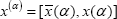 in Fig. 1), with the confidence degree indicating the level of belief that the concerned uncertain magnitude belongs in the corresponding interval (Klir and Yuan, 1995). This belief measure, called Necessity (Nec), is maximum for x⁽⁰⁾ (i.e.Nec(x⁽⁰⁾) = 1), because it is completely certain that the value of the magnitude is within the 0-cut, and decreases as α increases (shorter α-cuts). Specifically,

Nec(x^(α)) = 1 - α. (1)

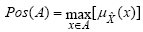
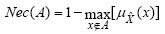
Necessity is defined for any set of real numbers (not only α-cuts x^(α)) with the aid of a related fuzzy measure called Possibility (Pos): In fact, for any given set A,

Pos(A) = 1 - Nec(A^c) (2)

Nec(A) = 1 - Nec(A^c) (3)

where, A^c is the complement of set A.

As this definition states, the Possibility that the concerned magnitude belongs to a set of points A (i.e. the Possibility of A itself) increases as the Necessity of being outside this set (i.e. in A^c) decreases, which is rather intuitive.

Furthermore, possibility theory states axiomatically that for any given pair of sets A and B, the Possibility associated to their union is the highest of their Possibilities:

Pos(A ∪ B) = max[Pos(A),Pos(B)]. (4)

In particular, for any interval of real numbers 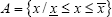, it can be written:

(5)

From these basic definitions, it follows that

(6)

for any real number x, where is the membership function of the fuzzy number (see Fig. 1).

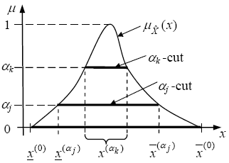
Fig. 1. Fuzzy number representation

Therefore, Possibility and Necessity of any real interval A can be evaluated from the membership function as:

	(7)
	(8)

These dual fuzzy measures are the basis of several techniques developed in areas such as decision-making under uncertainties. To this purpose, different ranking methods (Hamming distance, methods based on comparing α-cuts, methods based on the extension principle, etc.) have been proposed for comparing and ordering fuzzy numbers obtained, for example, with different scenarios.

B. Functions of Fuzzy Numbers

Given two fuzzy numbers and with α-cuts x^(α) and y^(α), and a real function of crisp variables: f(u,v), continuous in the domain u∈x⁽⁰⁾ and v∈y⁽⁰⁾, the fuzzy counterpart of f, is, according to the resolution principle, a fuzzy number whose α-cuts are the intervals:

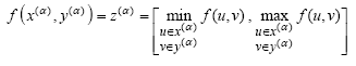(9)

This definition can be extended to functions of more than two independent variables.

Figure 2 illustrates the resolution principle. It can be seen that the α-cuts of are the images through f of the Cartesian product of the corresponding α-cuts of and . The same Necessity assigned to an α-cut of and is assigned to its image through f.

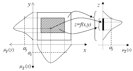
Fig. 2. Illustration of the resolution principle.

C. Systems of Fuzzy Equations

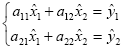
Interval equations, from which fuzzy equations come, arise as a direct generalization of their classical (crisp) counterpart when uncertain parameters are replaced by intervals containing all their possible values. Consider the following crisp linear system of equations:

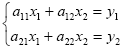(10)

If y₁ and y₂ are not exactly known but they are assumed to belong in the intervals and ], that is, and , a natural description of the situation is obtained replacing y₁ and y₂ by these intervals. That gives rise to the following system of interval equations, where the unknown are the intervals [] and []:

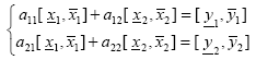(11)

Fuzzy equations arise when the intervals on the right-hand side are α-cuts of fuzzy numbers, and the corresponding interval solutions are assigned to the α-cuts of the fuzzy solution, i.e.:

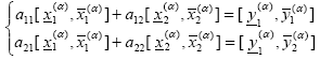(12)

or, in a more compact form:

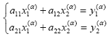(13)

A system of fuzzy equations brings together all these interval equations and is represented as:

(14)

More general cases exist, where some coefficients a_ij are also uncertain or where the equations are nonlinear.

In spite of their simplicity, interval equations have different kind of solutions depending on the meaning given to the equality sign in this context. Some relevant solution sets will be briefly described in the following. Interval equations will be considered in order to keep the explanation simple; however, each one has a fuzzy analogous where the intervals are α-cuts.

Interval Algebraic Solution (Classic Solution)

Referring to the two-dimensional case of Ec. (11), the Interval Algebraic Solution is the vector of intervals that fulfills both equations. As schematically shown in Fig. 3a, each equation maps all the points in the rectangle defined by the Interval Algebraic Solution (shaded area on the left) into its own right-hand side interval .

The fuzzy analogous of this interval solution is the Classic Fuzzy Solution on which previous fuzzy harmonic load-flow methodology relies (Hong et al., 2000). Two important characteristics of the Interval Algebraic Solution makes clear why a methodology based on Classic Fuzzy Solution are prone to underestimate and overestimate the voltage uncertainty:

1) Points within the domain defined by and ] (empty rectangle on the right of Fig. 3a) are not of concern in the context of the Interval Algebraic Solution. Actually, solution of the crisp Eq. 9 for a given point in this rectangle may not belong to the interval solution (shaded rectangle). Clearly this implies underestimation because when the right hand side intervals model inputs known with uncertainties (e.g. harmonic currents injected into different buses), all vectors in the right-hand side are possible, and the interval solution should consider all them.

2) The Interval Algebraic Solution not always exists, even for linear systems with non-singular coefficient matrices (this can be easily verified making, e.g. a₁₁= a₁₂= a₂₁ = 1, a₂₂= 0, , , and in Eq. (11). When the solution exists the upper and lower limits of the intervals , i= 1, 2,…, n, are the solutions of a linear system of 2n crisp equations, which coefficients matrix and right-hand side vector are particular arrangements of ±a_ij and ±y_i (Friedman et al., 1998). This system can always be set up, regardless of whether the Interval Algebraic Solution exists; when it does not, some of the intervals turn out to be unfeasible (i.e. ). The methodology based on the Classic Fuzzy Solution deals with this case reversing the improper intervals in order to get meaningful results called Weak Solutions (Friedman et al., 1998). However, these intervals are not actual solutions in the mathematical sense, and often overestimate the length of the proper intervals that can be obtained with the Hull Solution described below.

United Solution Set

While the Interval Algebraic Solution is a vector of intervals, the United Solution Set is the set of vectors schematically shown in Fig. 3b for the two-dimensional case. The set of solution vectors (shaded area in the [x₁, x₂] plane) is mapped by the matrix of elements a_ij in Eq. (11), into the rectangular domain defined by the intervals on the right-hand side. Conversely, this rectangular domain is mapped into the shaded area on the left by the inverse matrix (elements b_ij). Buckley and Qu (1991) proved that the Interval Algebraic Solution, if it exists, is a subset of the United Solution Set, as it is shown in the figure.

Hull Solution (Marginal Joint Solution)

Hull Solution is the interval analogous of the fuzzy Marginal Joint Solution (Reynaerts and Muzzioli, 2006) on which the proposed methodology is based. The Hull Solution is a vector of intervals. Specifically, given the matrix of coefficients a_ij in Eq. (11), and its inverse B=A^-1 of elements b_ij, the i^th component of the Hull Solution, , is the image of the rectangular domain defined by the intervals on the right-hand side through the i^th row of B.

This relationship is schematically shown in Fig. 3c, from which it is apparent that the rectangular domain defined by the components of the Hull Solution exactly encloses the United Solution, furthermore each component of the Hull Solution contains the corresponding component of the Interval Algebraic Solution (provided it exists).

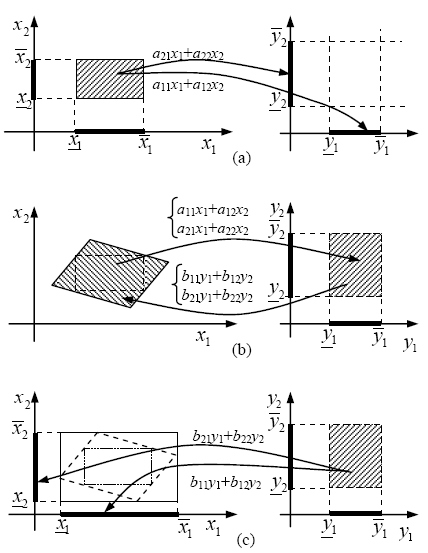
Fig. 3. Different kinds of solutions for a system of interval equations given by the α-cuts of a system of fuzzy equations;
(a) Interval Algebraic solution; (b) United Solution Set; (c) Hull Solution.

The Hull Solution (Marginal Joint Solution in the fuzzy context) provides the expected results in a harmonic load-flow analysis with uncertain parameters. In fact, we usually are not concerned with the set of voltage vectors produced by all the possible injected harmonic currents (United Solution Set), but only with the lower and upper value each harmonic bus voltage can reach, that is, the interval each component of the United Solution spans; just what the Hull Solution provides.

III. NEW PROPOSED FUZZY HARMONIC LOAD-FLOW

A. Aims and Assumptions

The following objectives and assumptions have been established for the developed methodology.

• Aims

1. Uncertainties in the harmonic impedances of linear loads have to be modeled in addition to those regarding harmonic currents injected by nonlinear loads.
2. Fuzzy harmonic voltage magnitudes have to be directly calculated. It will not be obtained from fuzzy real and imaginary components since possibilistic dependence would lead to overestimations.

• Assumptions

1. The fuzzy model is based on the deterministic harmonic penetration method (Heydt, 1994). Hence, nonlinear loads are modeled as injected harmonic currents independent from the voltage waveform. This hypothesis is quite reasonable in scenarios with low to moderate harmonic distortion, and is assumed in most of the harmonic load-flow programs. On the other hand, the accuracy of more sophisticated models (which take harmonic interaction into account) seems unnecessary in the context of uncertainties to which the proposed methodology is devoted.
2. Injected harmonic currents as well as admittances to ground that model linear loads are functions of uncertain parameters, e.g. firing angle of ac/dc converters, total active and reactive power, percentage of capacitive compensation, etc. Possibility of these uncertain parameters will be modeled through fuzzy numbers whose membership functions are assumed to be known and independent of each other.

B. Model formulation

Because of the first assumption above, the vectors of harmonic node voltage and injected currents are directly related through the nodal admittance matrix calculated at the corresponding harmonic frequency, i.e:

V^(h) = [Y^(h)]^-1I^(h) (15)

where h stands for the h^th harmonic order, and will be omitted from here on for notational simplicity. In this equation I is the vector of harmonic currents inject into the network by nonlinear loads. Its components depend on a set of parameters such as rated power of the nonlinear devices, firing angle, etc.

Let p_jk (k=1,…, np) be these parameters for the j^th component of I, so that it can be expressed as:

i_j = h_Ij(p_j1, ..., p_jk, ..., p_jnp); j = 1, ..., n, (16)

where function h_Ij depends on the specific model adopted for the nonlinear devices connected to this bus.

On the other hand, the linear load connected to the j^th bus is modeled as a grounded admittance, which only affects the j^th diagonal element of matrix [Y]. This admittance depends on the active and reactive power, percentage of induction motors in the load, capacitive compensation, etc. As in the case of p_jk and h_jk , let g_jk, k=1,…,ng and h_Yj be the parameter and the admittance function that model the linear load connected to node j, so that:

y_jj = h_Yj(g_j1, ..., g_jk, ..., g_jnp); j = 1, ..., n, (17)

By arranging the parameters p_jk and g_jk together in vectors G and P, Eq. (14) can be written as:

V(G,P) = [Y(G)] I(P) (18)

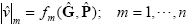
Let now

|v|_m = f_m(G,P); m = 1, ..., n (19)

be the expression of the voltage magnitude in node m, that is, the magnitude of m^th row in Eq. (18).

When uncertainties in the components of G and P are modeled as fuzzy numbers, |v|_m also becomes fuzzy:

(20)

and its α-cuts are the image of the corresponding α-cuts of P and G through f_m:

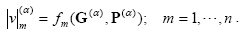(21)

According to Eq. (21), the lower and upper limits of are the minimum and the maximum values that f_m reaches when the elements of G and P varies in their respective intervals in G^(α) and P^(α).

Nonlinear programming techniques based on gradient methods are used to find these limits for a set of decreasing α-cuts, starting from α₁=1 to α_N=0. Initial guesses for the iterative process in the α_k-cut are the values that minimize and maximize |v|_m in the α_k-1-cut.

In each step of the iterative nonlinear programming algorithm, partial derivatives of f_m respect each parameter p_jk and g_jk have to be calculated for specific values of these variables. Eq. (22) and (23) provide computationally suitable expressions for this calculation, making the nonlinear programming approach efficient:

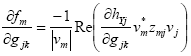	(22)
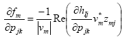	(23)

In these equations z_mj are the elements of [(ZG)] = Y(G)]^-1, and v_m^* is the complex conjugate of the voltage at bus m. The admittance matrix [Y] and the vector of injected currents I are obtained for the required set of parameters g_jk and p_jk . Then the impedance matrix [Z]=[Y]^-1 and the vector of complex node voltages V=[Z]I are computed in order to obtain v_m^*.

The scalar partial derivatives and clearly depend on the models implemented for the linear and nonlinear loads (Eq. (16) and (17)).

IV. VALIDATION OF THE METHODOLOGY

A. Test System Description

The system of Fig. 4, which is based on the well-known 14-bus harmonic test system from IEEE (Abu-Hashim et al., 1999), will be used to assess the main features of the proposed methodology. To this purpose, the results obtained with the new methodology will be compared with those obtained with the fuzzy methodology based on the Classic Fuzzy Solution and with Monte Carlo simulations.

The IEEE test system data, available at http://www.ee.ualberta.ca/pwrsys/harmonics.html, have been used except for the assumed uncertain parameters detailed below.

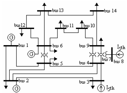
Fig. 4. 14-bus standard test system for harmonic analysis.

Uncertain Nonlinear loads

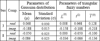
Triangular fuzzy numbers have been used to model possibility distributions of the real and imaginary components of the harmonic currents injected by nonlinear loads, whereas Gaussian distributions truncated at two standard deviations have been chosen to model the probabilistic counterpart in Monte Carlo simulations.

Table 1 shows the parameters of the possibilistic and probabilistic distributions. Note that the shapes and parameters of possibilistic and probabilistic models fulfill the necessary coherence between possibilistic and probabilistic information: 1) all probable values of input variables are also possible, 2) non-possible values have zero probability 3) the most possible value matches the mode.

Uncertain Linear loads

The frequency dependence of impedances used to model linear loads has been represented according to the 3^rd model recommended by CIGRE (1981).

In cases where uncertain linear loads have been assumed, they have been modeled through independent triangular fuzzy numbers, centered at the standard values in the IEEE test case, and varying ±10% around them in their 0-cuts. Similarly to the nonlinear load model, coherence with probabilistic information was assured using normal distributions truncated at 2σ, with mean (μ) matching the most possible values and standard deviations σ = 0.05μ.

Table 1: Per unit 5th order harmonic currents injected into the system (nonlinear loads models)

B. Simulation Results and Analysis

Figure 5 shows the histogram and membership functions of the 5^thorder per unit harmonic voltages at buses 1, 3 and 9, calculated through Monte Carlo simulation, the proposed methodology and the possibilistic approach based on the Classic Fuzzy Solution (Hong et al., 2000).

In order to compare the results, and since the methodology based on Classic Fuzzy Solution is not able to model uncertainties in linear loads, it was assumed that active and reactive power of linear loads are crisp values in all the simulations shown. On the other hand, fuzzy arithmetic was applied to calculate fuzzy voltage magnitudes from the real and imaginary components given by the Classic Fuzzy Solution.

Figure 6 shows the same variables as Fig. 5, although in this case the uncertainties in linear load parameters were considered (Classic Solution approach is not applied in this case).

Although quantitative comparison between possibilistic and probabilistic measures of uncertainty is not possible, Fig. 5a and 5b as well as 6a and 6b, show a good qualitative agreement among results obtained with the proposed methodology and with Monte Carlo simulations. Comparison of Fig. 5b and 6b, shows that the uncertainty in harmonic voltages increases as expected when the uncertainties in linear loads are modeled. In fact, Fig. 7 demonstrates clearly this influence showing the 5^th harmonic voltage at bus 3 when linear load variations are known with of uncertainties of 0%, ±10% and ±20%. It should be pointed out that modeling linear loads uncertainties could be even more important for higher harmonics orders (Burch et al., 2003).

On the other hand, as it is expected, the developed model and the probabilistic Monte Carlo simulation keep in their outputs the coherence imposed to their input variables: 1) all probable values of the harmonic voltages are also possible, 2) non-possible values have zero probability, 3) the most possible value matches the mean¹.

Clearly, over- and underestimation of the harmonic voltage uncertainties shown by the Classic Fuzzy Solution approach in Fig. 5c do not occur with the methodology based on the Marginal Joint Solution.

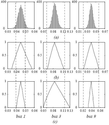
Fig. 5. Per unit 5^th order harmonic voltage magnitude at buses 1, 3 and 9. Case considering certain linear loads
(a) Histogram from Monte Carlo simulation.
(b) Fuzzy voltages from the proposed fuzzy approach.
(c) Fuzzy voltages from Classic Fuzzy Solution methodology.

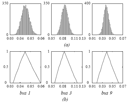
Fig. 6. Per unit 5^th-harmonic voltage magnitude at buses 1, 3 and 9. Case considering uncertain linear loads
(a) Histogram from Monte Carlo simulation.
(b) Fuzzy voltages from the proposed fuzzy approach.

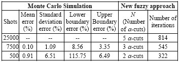
Finally, in order to compare the computational effort of the new fuzzy approach regarding Monte Carlo Simulation, the number of iterations² considering three cases with N= 2, 3 and 5 α-cuts, starting from α₁ = 1 to α_N = 0, were taking into account; i.e. two α-cuts permit to obtain an approximate fuzzy number. On the other hand, Monte Carlo simulations were computed after 500, 7500 and 25000 iterations; additionally the highest errors in mean, standard deviation, minimum and maximum boundaries with respect to the 25000 shots case were established and reported in Table 2.

Monte Carlo simulation errors reported in Table 2 suggest that at least 7500 or more deterministic simulations are necessaries to obtain representative results of the system, as a consequence, it is clear that Monte Carlo simulation is a computationally expensive method; even more than the new fuzzy approach evaluating five (5) α-cuts at each fuzzy parameter since it only needs 814 deterministic simulations to achieve the results.

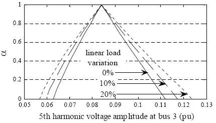
Fig. 7. Fuzzy voltage at bus 3 for different ranges of linear load variations.

Table 2: Number of deterministic iterations to achieve the solution.

V. CONCLUSIONS

Possibility theory arises as a powerful tool to deal with parameters which nature is imprecise, vague, fuzzy, and so on, and which cannot be described in probabilistic term. This is often, in practice, the case of harmonic load-flow studies. In this sense, recently, a fuzzy harmonic load-flow calculation method was proposed by Hong et al., 2000; however, the Classic Fuzzy Solution on which that method relies exhibits some drawbacks, i.e., harmonic voltage over- and underestimation and incapability to model uncertainty in linear loads. This latter represent a strong weakness, because linear loads are usually not well known, and significantly affect the harmonic impedances in the system, thus also the harmonic load-flow.

To overcome these drawbacks, a new possibilistic methodology for harmonic load-flow calculation based on fuzzy sets theory has been presented in this article. This approach allows including fuzzy models for the uncertainties in both linear and nonlinear loads. In addition, because the Marginal Joint Solution is obtained, the methodology avoids under-and overestimation of the harmonic voltages.

Nonlinear programming techniques have been applied to establish the Marginal Joint Solution.

In order to evaluate the performance of the new fuzzy methodology, a comparison with Monte Carlo simulations (assuming availability of statistical information to model uncertain parameters) was developed. Tests reported show that results obtained with both methodologies are in good agreement, in fact, even though no direct quantitative comparison of uncertainty measures is possible between fuzzy numbers and probabilistic distributions, results provided by both methodologies can lead to a similar qualitative assessment. On the other hand, from a computational point of view, thousands of Monte Carlo simulation shots were necessaries to achieve similar extreme values of harmonic voltages to those obtained from the new fuzzy approach. In this sense, the new fuzzy method exhibits a better computational performance, if it is considered that results are achieved with much less computational effort. This computational advantage could be even more important when large electric power systems are assessed.

The new fuzzy harmonic load-flow represents a useful tool to make decisions under uncertainty, especially, in studies such as: harmonic filters design, capacitors locating, impact of a new harmonic load connection, and so on. The main advantage of the new approach is just that it permits to model linear and nonlinear load input parameters which, in real power systems, are not really random in nature but imprecisely known.

---

¹ Actually, since the histograms obtained from Monte Carlo simulations regard to samples of the complete populations, consistency is only partially, although forcefully, demonstrated.
² Each iteration implies the solution of a deterministic system of equations as expressed in Eq. 15

REFERENCES
1. Abu-Hashim, R., R. Burch, G. Chang, M. Grady, E. Gunther, M. Halpin, C. Harziadonin, Y. Liu, M. Marz, T. Ortmeyer, V. Rajagopalan, S. Ranade, P. Ribeiro, T. Sim and W. Xu, "Test Systems for Harmonics Modeling and Simulation", IEEE Trans. On Power Delivery, 14, 579-585 (1999).         [ Links ]
2. Baghzouz, Y., R.F. Burch, A. Capasso, A. Cavallini, A.E. Emanuel, M. Halpin, R. Langella, G. Montanari, K.J. Olejniczak, P. Ribeiro, S. Rios-Marcuello, F. Ruggiero, R. Thallam, A. Testa and P. Verde, "Time-Varying Harmonics: Part II - Harmonic Summation and Propagation", IEEE Trans. Power Delivery, 17, 279-285 (2002).         [ Links ]
3. Bukcley, J., and Y. Qu, "Solving Systems of Linear Fuzzy Equations", Fuzzy Sets and Systems; 43, 33-43 (1991).         [ Links ]
4. Burch, R., G. Chang, C. Hatziadoniu, M. Grady, Y. Liu, M. Marz, T. Ortmeyer, S. Ranade, P. Ribeiro and W. Xu, "Impact of Aggregate Linear Load Modeling on Harmonic Analysis: A Comparison of Common Practice and Analytical Models", IEEE Trans. Power Delivery, 18, 625-630 (2003).         [ Links ]
5. Chan, W.L., H. Hon and T. P. Albert, "Fuzzy Arithmetic Based Power Harmonics Signature Recognition", IEE 2nd International Conf. on Advances in Power System Control (1993).         [ Links ]
6. CIGRE Working Group 36-05, "Harmonics, Characteristic Parameters, Methods of Study, Estimates of Existing Values in the Network", Electra, 77, 35-54 (1981).         [ Links ]
7. Dimitrovski, A., and K. Tomsovic, "Boundary Load Flow Solutions", IEEE Transactions on Power Systems, 19, 348-355 (2004).         [ Links ]
8. Esposito, T., G. Carpinelli, P. Varilone and P. Verde, "First-order Probabilistic Harmonic Power Flow", IEEE Proc.-Generat., Trans. and Dist., 148, 541-548 (2001a).         [ Links ]
9. Esposito, T., G. Carpinelli, F. Rossi and P. Verde, "Probabilistic Harmonic Power Flow for Percentile Evaluation", Conf. on Electrical and Computer Eng., 2, 831-838 (2001b).         [ Links ]
10. Friedman, M., M. Ming and A. Kandel, "Fuzzy Linear Systems", Fuzzy Sets and Syst., 96, 201-209 (1998).         [ Links ]
11. Heydt, G.T., Electric Power Quality, Stars in a Circle, Publications (1994).         [ Links ]
12. Hong, Y., J. Lin and C. Liu, "Fuzzy Harmonic Power Flow Analyses", Inter. Conf. on Power System Tech., 1, 121-125 (2000).         [ Links ]
13. Klir, G.J. and Y. Bo, Fuzzy Sets and Fuzzy Logic, theory and applications, Prentice Hall (1995).         [ Links ]
14. Miranda, V., M. Matos and J. Saraiva, "Fuzzy Load Flow - New Algorithms Incorporating Uncertain Generation and Load Representation"; Inst. de Eng. De Sist. e Comp. - INESC and Fac. Eng. Univ. Porto - FEUP/DEEC (1990).         [ Links ]
15. Reynaerts, H. and S. Muzzioli, "Fuzzy Linear Systems of the form A1x+b1=A2x+b2", Fuzzy Sets and Systems; 157, 939-951 (2006).         [ Links ]

Received: October 6, 2006.
Accepted: October 24, 2007.
Recommended by Subject Editor Julio Braslavsky.