


Servicios Personalizados
Revista

Articulo
 Inglés (pdf)
 Articulo en XML
 Referencias del artículo
 Enviar articulo por email
Indicadores
-
 Citado por SciELO
Links relacionados
-
 Similares en
SciELO
Similares en
SciELO
Compartir

 Permalink
Latin American applied research
versión impresa ISSN 0327-0793
Lat. Am. appl. res. vol.39 no.1 Bahía Blanca ene. 2009
ARTICLES
Optimal tuning parameters of the dynamic matrix predictive controller with constraints
G.M. De Almeida, J.L.F. Salles and J.D. Filho
UFES -Univ. Federal do Espirito Santo - Departmento de Eng. Elétrica
Av. Fernando Ferrari C. P. 019001 - Vitória, ES, Brasil
gmaialmeida@yahoo.com.br, jleandro@ele.ufes.br, jdenti@ele.ufes.br
Abstract -Dynamic Matrix Control Algorithm is a powerful control method widely applied to industrial processes. The idea of this work is to use the Genetic Algorithms (GA) with the elitism strategy to optimize the tuning parameters of the Dynamic Matrix Controller for SISO (single-input single-output) and MIMO (multi-input multi-output) processes with constraints. A comparison is made between the computational method proposed here with the tuning guidelines described in the literature, showing advantages of the GA method.
Keywords -Genetic Algorithm. Dynamic Matrix Control. Automatic Tuning. Constraints Management.
I. INTRODUCTION
Model Predictive Control (MPC) refers to a class of computer control algorithms that utilize an explicit process model to predict the future response of the plant (Qin and Badgwell, 2003). A variety of processes, ranging from those with simple dynamics to those with long delay times, non-minimum phase zeros, or unstable dynamics, can all be controlled using MPC. MPC integrates optimal, stochastic, multivariable, constrained control with dead time processes to represent time domain control problems (see Camacho and Bordons, 2004; Maciejowski, 2002; and Rossiter; 2003).
The MPC algorithms usually exhibit very good performance and robustness provided that the tuning parameters (prediction and control horizons and move suppression coefficient) have been properly selected. However, the selection of these parameters is challenging because they affect the close loop time response, being able to violate the constraints of the manipulated and controlled variables. In the past, systematic trial-and-error tuning procedures have been proposed (see Maurath et al., 1988; Rawlings and Muske, 1993; and Lee and Yu, 1994). Recently there are some works proposing alternative techniques of adjusting then automatically. In Filali and Wertz (2001) and Almeida et al. (2006) it was used the Genetic Algorithms (GA) to design the tuning parameters of the Generalized Predictive Control (GPC) applied in SISO and time-varying systems without constraints. Another tuning strategy that can be implemented in a computer was proposed by Dougherty and Cooper (2003) which developed easy-to-use tuning guidelines for the Dynamic Matrix Control (DMC) algorithm, one of the most popular MPC algorithm in the industry. DMC uses the step response to model the process, and it is also applied in SISO and MIMO processes that can be approximated by first order plus dead time models.
The main goal of this work is to tune the DMC controller parameters for SISO and MIMO dynamical systems with input and output constraints using GA, in order to optimize the time response specifications (overshoot, rise time and steady state error) and to guarantee feasibility of solutions. It also carries through a comparative study between the method proposed here and the tuning guidelines proposed by Dougherty and Cooper (2003).
This paper is organized as follows: Section 2 describes the classical formulation of the DMC algorithm with constraints and presents the automatic tuning guidelines proposed by Dougherty and Cooper (2003); Section 3 makes an overview of GA and shows the application of GA with elitism strategy for tuning of the DMC parameters; in Section 4 we make the comparison between the proposed method here and the method described in the literature; Section 5 presents the conclusions.
II. DYNAMIC MATRIX CONTROL (DMC)
In this section we formulate the predictive control problem and we present its solution from the DMC algorithm.
Let us consider a linear MIMO dynamic system with m inputs (ul, l =1,...,m) and n outputs (yj, j =1,...,n), that can be described by the expression:
 | (1) |
where gjl is the step response of output j with respect to the input l, and ?ul(k)= ul(k)-ul(k-1), is the control signal variation. Let us denote by  the i step ahead prediction of the output j from the actual instant k; and rj(k+i) is the i step ahead prediction of the set point with respect to the output j.
The basic idea of DMC is to calculate the future control signals along the control horizon hc, i.e., determine the sequence ul(k+i), for l = 1, 2,...,m and i = 0,..., hc - 1, in such a way that it minimizes the cost function defined by:
 | (2) |
where λj is the move suppression parameter and hp is the prediction horizon. In addition, the following constraints must be satisfied for l =1,...,m and j =1,...,n:
 | (3) |
Considering ?ul(k+i)=0,i > hc,i ≥ 1, and assuming that exists an integer number Ns such that ?ul(k)=0 for k > Ns, and l=1, ..., m, the predictive output form the actual instant k is given by the following convolution:
 | (4) |
Disconnecting in (4) the future control actions (?ul(k+i); i>1) from the past control actions, and de?ning:
 | (5) |
we can represent the expression (4) by:
 | (6) |
where the first term in expression (6) is the forced response, that depends on the present and future control actions, and the second is the free response, that depends on the past control actions.
In the sequel we formulate the control problem as a standard quadratic programming problem with constraint. Let us define the following vectors:
 | (7) |
Using the definitions above, we can represent the m predicted outputs along the prediction horizon hp by the expression:
 | (8) |
where  has dimension nhp × mhc and is given by:
 | (8) |
Let us denote by  a m×m diagonal matrix with move suppression parameters λj, j =1 ,..., m, on its diagional, and let
  a mhc × mhc matrix defined by:

From (8), we can represent the cost function (2) by the following expression:
 | (9) |
where  ,
,  and
and  .
.
Applying recursively the fact that ul(k+i) = ul(k+i-1)+ ?ul(k+i-1) in the second restriction of (3) and considering (4) in the third inequality of (3), we conclude that (3) is equivalent to:
 | (10) |
The solution of the Predictive DMC control problem is divided in two step: first we calculate the prediction vector  by minimizing the quadratic function (9) with 2mhc + nhp constraints given in (10). Next we apply the current signal ?u(k) in the input of the processes and we discard the future signals ?u(k+i), i =1,...,hc - 1 (this is called receding horizon control technique).
A. Comments about the DMC parameters
The relative importance of each one term in the cost function (2) can be reinforced by increasing the move suppression parameter (λj), the control horizon (hc) and the prediction horizon (hp) (Garcia et al., 1988). However the increment in these parameters affects the time response of the output y(k) (overshoot, rise time and steady state error; Garcia et al., 1988).
An increment in the parameter λj decreases the control variables, making the time response slower and softer. The variations in this parameter also affects the robustness of the DMC controller (the increment in the parameter λj increases the robustness; Georgeou et al., 1988).
An increment in the control horizon (and consequently in the prediction horizon, since hc≤hp), makes an improvement in the performance of the DMC controller, increasing the controlled variables, but decreasing the robustness of the controller, (see Georgeou et al., 1988). It is also observed in Georgeou et al. (1988) that the tuning of the parameter λj by keeping fixed the control and prediction horizons does not lead to good results; but the contrary case makes the adjustment more feasible. This fact shows that the prediction and the control horizons have a higher adjustment priority than the parameter λj.
It is also observed that the constraint in the control signal variations (?u) affects directly the speed of the output response and this constraint has an higher adjustment priority than the parameter λj, (see Prett and Garcia, 1988). On the other hand, the constraints in the quadratic programming problem increase proportionally with the prediction and control horizons, increasing the complexity of the calculations which favor the obtainment of unfeasible solutions. Thus, it is so important to consider these facts to make the best tuning of the DMC parameters.
B. Tuning Guidelines
The methods encountered in the literature for tuning the DMC parameters are mostly based on heuristic rules and trial and error, see Camacho and Bordons (2004) and Maciejowski (2002). Only in Dougherty and Cooper (2003) is derived an analytic expression to determine the move suppression parameter λj for mono and multivariable systems, in order to obtain an automatic tuning method. The guidelines proposed by Dougherty and Cooper (2003) is described in next steps:
Step 1. Approximate the process dynamics of controller output to measured controlled variables pairs of non-integrating sub-processes with the first order plus dead time (FOPDT) model:

for l =1, 2,..., m; j =1, 2,...,n.
Step 2. Select the sample time as close as possible to:

Step 3. Compute the prediction horizon, hp, and the model horizon Ns:

where  .
.
Step 4. Compute the control horizon, hc

Step 5. Select the controlled variable weights,  , to scale the process unit to be the same.
Step 6. Compute the move suppression coefficient,
 | (11) |
Step 7. Implement DMC using the traditional step response matrix of the actual process and the initial values of the parameters computed in steps 1-6.
III. GENETIC ALGORITHMS
Genetic algorithms were first presented by Holland (1975) and are based on the mechanics of natural selection of Darwin and the natural genetics of Mendel. They are a parallel global search technique that emulate natural genetic operators and work on a population representing different parameter vectors whose optimal value with respect to some criterion (fitness) is searched. This technique includes operations such as reproduction, crossover and mutation. These operators work with a number of artificial creatures called generation. By exchanging the information of each individual in a population, GA preserves the best individual and yields higher fitness in each generation such that the performance can be improved. The basic operators of GA are:
Crossover: This operation provides a mechanism to exchange the information of the individuals via probabilistic process. This operation takes two "parents" individuals and produces two "off-springs" which are new individuals whose characteristics are a combination of those of their parents. The operation of crossover can be seen in the Fig. 1.

Figure 1: Crossover Operation
Mutation: Mutation is an operation where some characteristics of an individual are randomly modified, yielding a new individual. Here, the operation simply consists in changing the value of one bit of the string representing an individual in a random way. This operation is shown in the Fig. 2.

Figure 2: Mutation Operation
Reproduction: Reproduction is the process in which a new generation is obtained by selecting individuals from an existing population, according to their fitness. It takes one or more copies of the individuals with higher fitness values in the next generation, while individuals with lower fitness may have none. Note, however, that reproduction does not generate new individuals but only favors the percentage of fittest individuals in a population of given size (it is called elitism strategy). The Fig. 3 shows the reproduction operator.
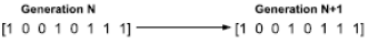
Figure 3: Reproduction Operation
A. Convergence of the Genetic Algorithm
In the field of GA and convergence behavior, we could distinguish two large areas of research. The first line of research results from the theoretical investigations by Holland (1975) and Goldgerb (1989) and is based on the schemata theorem and the Walsh functional analysis. However, the global searches of crossover and mutation are not considered possible under the schemata theorem. In addition the Walsh functional analysis has been used to evaluate the "phenomenon of deception", but it can never analysis the general behavior of GAs. The second line of research treats GAs as a Markov Chain, (see Schafer and Telega, 2007). In Rudolph (1997), it is proved the global convergence of GA algorithm with the elitism strategy and in Schmitt and Rothlauf (2001) it is investigated the determinants which the convergence rate depends on. They showed that it depends mainly on the value of the second largest eigenvalue of the transition matrix of the Markov Chain. However the authors could not explain how this matrix is affected by the GA parameters, like mutation and crossover rates, in order to improve the convergence of GA algorithm. There are a great deal of discussions of parameter settings and approaches to parameters adaptation in the evolutionary computation literature. In Srinivas and Patnaik (1994) it is heuristically proposed that the population size, the crossover rate and the mutation rate must lie in the intervals [30,200], [0.5,1.0] and [0.001,0.05], respectively.
B. Tuning by GA
The individual of GA is given by the vector of tuning parameters [hp,hc,λ1,..., λm] .For each one we associate the fitness function given by:
 | (12) |
where yj is the output, rj is the set point, Sc is the set of constraints given in (10) and 1{x∈A} is the indicator function of a set A, i.e., if x∈A then 1{x∈A} =1, otherwise 1{x∈A} =0. The first term in (12) is the inverse of the integrated square-error (ISE) and the second term penalizes the unfeasible solutions.
Next the GA program calculates the fitness function of each individual and selects the best parents according to the roulette wheel method. Then, it generates the new individuals by executing the crossover, mutation and reproduction operators. The procedure is summarized in the following steps:
Step 1: Define the population size, the maximum generation, the crossover rate and the mutation rate;
Step 2: Create an initial population;
Step 3: Calculate ?u(k) by solving the Linear Quadratic Programming problem defined by the function (9) and the constraints (10);
Step 4: Calculate the fitness of each individual from (12);
Step 5: Select the parents individuals from the roulette wheel method;
Step 6: Create a new population by applying the genetic operators (crossover, mutation and reproduction);
Step 7: Go to step 3 until the maximum generation is reached.
IV. NUMERICAL RESULTS
In this section we compare the Guideline method presented in Section II.B with the tuning method proposed in section III.B. The algorithms were implemented in a Pentium Processor with 2.8 GHZ and 512 MB. We used the MatLab 7.0 and the optimization problem was solved by the Quadriprog routine. We apply the DMC algorithm in SISO and MIMO systems with constraints in the control action (u(k)), in the control signal variation (?u(k)) and in the output response (y(k)). These constraints are:
 | (13) |
The population generated by the GA program has 50 individuals and the rates of crossover, mutation and reproduction are equal to 0.8, 0.01 and 0.1, respectively.
A. SISO System
The first example is a first order plus dead time model, represented by the transfer function:
 | (14) |
The Table 1 compares the tuning parameters (hp,hc,λ) and the total number of constraints (NC) in the quadratic programming problem determined by both methods. We observe from (10) that NC=2mhc+nhp, where n and m are the number of output and control signals respectively. The Fig. 4 presents the time responses of signals y(t),u(t) and ?u(t) by considering the step input and the parameters in Table 1.
Table 1: Simulations for SISO system


Figure 4: Time Responses of signals y, u and ?u
The Fig. 5 shows the evolution of the mean fitness of the population at each generation. We observe that it converges to the fittest individual at the twentieth generation, which characterizes a global convergence of the Genetic Algorithm with the elitism strategy as we discussed in Section 3.A. The time for convergence of the proposed algorithm in Section 3.B is about 101.3 s. for the SISO system and 119.12 s. for the MIMO system. The half of these processing time is spent by the Quadriprog routine (step 3 in the algorithm of Section 3.B).

Figure 5: Convergence of the mean fitness
B. MIMO System
The second example exhibits a multivariable system with two inputs (m = 2) and two outputs (n = 2), represented by the transfer function matrix
 | (15) |
The Table 2 compares the tuning parameters and the total number of constraints (NC) for the MIMO system. The Figs. 6 and 7 show the time response presented by both methods, considering the step input and the tuning parameters described in the Table 2.
We observe in Tables 1 and 2 that the GA method furnishes lesser prediction and control horizons than the Tuning Guidelines. Thus, from the comments in Section 2.A, we conclude that the DMC algorithm tuned by GA is more robust with respect to the variations in the model parameters than the DMC algorithm tuned by the Guidelines method (despite of sometimes the parameter λ furnished by the guidelines method be larger than that given by the GA method). This can be illustrated in Table 3 where we compare the ISE index of the SISO system for both tuning methods when the gain K = 3 of the model is changed.
Table 2: Simulations for MIMO System

Table 3: ISE index of the SISO system


Figure 6: Time Responses of y1,u1 and ?u1

Figure 7: Time Responses of signals y2,u2 and ?u2
In addition, the DMC algorithm tuned by the GA method has lower number of constraints in the quadratic optimization problem. In view of this, we observe in the time responses of signal y illustrated in the Figs. 4, 6 and 7 that the DMC controllers tuned by the literature Guidelines give non feasible solutions, since the controlled outputs y exceed the constraints (13).
V. CONCLUSIONS
The comparative study made in this paper, between the two automatic tuning methods, allowed us to conclude important advantages in favor of GA with the elitism strategy. The first is that it generated a lesser number of control and prediction horizons, improving the robustness of the DMC controller without the depreciation of the step time response (overshoot, rise time and steady state error). The second is that the GA method gave a lesser number of constraints in the quadratic programming problem, implying in a lower computational effort to solve the predictive control problem. The third is that the GA method reaches the feasible solutions more easily. In fact, an extreme number of constraints in the DMC algorithm can inhibit its application to real situations where the processing time is crucial, such as those found in the aerospace and robotic areas. In addition, a successful controller for the process industries must maintain the system as close as possible to the constraints, without violating then. The advantages exposed here can be extended to the Generalized Predictive Controller tuned by GA.
REFERENCES
1. Almeida, G., J. Salles and J. Filho, "Using genetic algorithms for tuning the parameters of generalized predictive control," VII Conferência Internacional de Aplicações Industriais INDUSCON, Recife (2006). [ Links ]
2. Camacho, E.F. and C. Bordons, Model Predictive Control, Springer, New York (2004). [ Links ]
3. Dougherty, D. and D. Cooper, "Tuning Guidelines of a Dynamic Matrix Controller for Integrating (Non-Self-Regulating) Processes," Ind. Eng. Chem. Res. 42, 1739-1752 (2003). [ Links ]
4. Filali, S. and V. Wertz, "Using genetic algorithms to optimize the design parameters of generalized predictive controllers," International Journal of Systems Science 32, 503-512 (2001). [ Links ]
5. Garcia, C., D. Prett and B. Ramaker, "Fundamental Process Control," The Second Shell Process Control Workshop, Butterworths, Stoneham, MA., 401-440 (1988). [ Links ]
6. Georgeou, A., C. Georgakis and W.L. Luyben, "Nonlinear Dynamic Matrix Control for High-Purity Destilation Columns," AIChE Journal, 34, 1287-1298, (1988). [ Links ]
7. Goldgerb, D.E., Genetic algorithms in search, optimization, and machine learning, Addison-Wesley. Ann Arbor (1989). [ Links ]
8. Holland, J.H., Adaptation in natural and artifficial systems, The University of Michigan Press, Ann Arbor, Berlin (1975). [ Links ]
9. Lee, J. and Z. Yu, "Tuning of Model Predictive Controller for Robust Performance," Computers and Chem. Eng. 18, 15-37 (1994). [ Links ]
10. Maciejowski, J., Predictive Control with Constraints, Englewood Cliffs, NJ, Prentice Hall (2002). [ Links ]
11. Maurath, P., D. Mellichamp and D. Seborg, "Predictive Controller Design for Single Input/Single Output Systems," Ind. Eng. Chem. Res. 27, 956-963 (1988). [ Links ]
12. Prett, D. and C. Garcia, Fundamental Process Control, Butterworths, Stoneham, MA (1988). [ Links ]
13. Qin, S. and T. Badgwell, "A Survey of Industrial Model Predictive Control Technology," Control Engineering Practices, 11, 733- 764 (2003). [ Links ]
14. Rawlings, J. and K. Muske, "The Stability of Constrained Recending Horizon Control," IEEE Trans. Autom. Control, 38, 1512-1516 (1993). [ Links ]
15. Rossiter, J.A., Model-Based Predictive Control: A Pratical Approach, CRC Press, Boca Raton, FL (2003). [ Links ]
16. Rudolph, G., Convergence properties of evolutionary algorithms, Springer, New York, Kovac, Hamburg (1997). [ Links ]
17. Schafer, R. and H. Telega, Foundations of Global Genetic Optimization, Springer Verlag, Berlin Heidelberg (2007). [ Links ]
18. Schmitt, F. and F. Rothlauf, "On the mean of the second larges of the second largest eigenvalue on the convergence rate of genetic algorithms," Working paper in Information Systems, University of Bayreuth, Germany (2001). [ Links ]
19. Srinivas, M. and L.M. Patnaik, "Genetic Algorithms: A Survey," IEEE Computer, 27, 17-26 (1994). [ Links ]
Received: November 22, 2007.
Accepted: May 8, 2008.
Recommended by Subject Editor José Guivant.

