ARTICLES

An h-adaptive unstructured mesh refinement strategy for unsteady problems

G. A. Rios Rodriguez, N. M. Nigro and M. A. Storti

Centro Internacional de Métodos Computacionales en Ingeniería CIMEC
Universidad Nacional del Litoral, CONICET
Güemes 3450, 3000, Santa Fe, Argentina
gusadrr@yahoo.com.ar, mstorti@intec.unl.edu.ar

Abstract - An h-adaptive unstructured mesh refinement strategy to solve unsteady problems by the finite element method is presented. The maximum level of refinement for the mesh is prescribed beforehand. The core operation of the strategy, namely the refinement of the elements, is described in detail. It is shown through numerical tests that one of the advantages of the chosen refinement procedure is to keep bounded the mesh quality. The type of element is not changed and no transition templates are used, therefore hanging nodes appear in the adapted mesh. The 1-irregular nodes refinement constraint is applied and the refinement process driven by this criterion is recursive. Both the strength and weakness of the adaptivity algorithm are mentioned, based on clock time measures and implementation issues. To show the proper working of the strategy, an axisymmetric, compressible non-viscous starting flow in a bell-shaped nozzle is solved over an unstructured mesh of hexahedra.

Keywords - H-Adaptivity; Unstructured Meshes; Quality Metrics; Hanging Nodes.

I. INTRODUCTION

The benefits of mesh adaptivity in the solution of Computational Fluid Dynamics problems by the Finite Element Method are well recognized. Amongst them, h-adaptive or mesh enrichment procedures have the advantage that they do not need to modify the fluid dynamic solver to be used.

The development of an h-adaptive element-based unstructured mesh strategy to solve unsteady problems by the finite element method is described in this work. It can be applied both to two- and three-dimensional unstructured linear finite element meshes. The adaptivity algorithm is designed considering the element refinement stage as the core of the strategy. This allows to extend the algorithm from 2-D meshes to 3-D ones with little extra effort. The refinement algorithm has been successfully tested by Rios Rodriguez et al. (2005), solving steady fluid dynamic problems on meshes made up of triangles, quadrangles and tetrahedra. Special care has been taken to keep bounded the quality decrease of the mesh. Edge midpoints or regular 1:4 and 1:8 refinement seems to be the best choice in this sense, for two- and three-dimensional elements correspondingly. It is also shown based on numerical tests that the best choice (from the quality standpoint) to regularly refine a tetrahedron in 8 sub-tetrahedra is to choose the shortest diagonal of the inner octaedron that arises in the partitioning process. Hanging nodes have to be managed since no transition elements are used to match zones of different refinement levels. To ensure a smooth transition in element size between zones with different levels of refinement, the 1-irregular node constraint amongst neighboring elements is considered. Consequently, the refinement process is recursively designed and the solution must be constrained on these hanging nodes. The selection method of the elements to be refined is shortly described as well. In this work, the strategy is used to solve the unsteady starting flow in a bell-shaped rocket nozzle over an unstructured mesh of hexahedra. While the adaptivity software runs on a single processor, the fluid dynamic problem solver developed by Storti et al. (1997-1999) runs in parallel on a Beowulf cluster. To show the algorithm efficiency, clock time is measured using a uniformly refined mesh equivalent to the adapted one. Finally, the advantages as well as the disadvantages of the strategy are highlighted.

II. ELEMENT REFINEMENT

It is considered that the main issue in the design of the refinement algorithm is to minimize the quality drop of the adapted mesh, since high quality meshes are often desired for numerical reasons. Computational cost and programming simplicity are also taken into account in the process design. If a regular 1:8 tetrahedron refinement is applied, four similar subtetrahedra are obtained at the corners of the parent element and an inner octahedron results. By adding an edge, the octahedron can be splitted into four tetrahedra, as Fig. 1 shows.

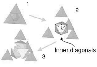
Figure 1: Regular 1:8 tetrahedron refinement sequence.

One of the three possible diagonals must be chosen (these diagonals are marked as dashed lines in Fig. 1). Usually, the diagonal is chosen randomly but it will be shown through numerical tests that there is a better choice.

A. Quality Tests

Several tetrahedron shape measures exist in the literature. Some of them are based on geometrical properties of the element while others are related to algebraic properties of the Jacobian matrix and the matrices thereof derived. Knupp (2001) defined the concept of algebraic mesh quality metrics and introduced a complete list of them. Here, it is considered that the quality of the mesh is equal to that of its most poorly-shaped element. The tetrahedron quality is measured using both the minimum dihedral angle and the algebraic shape measure introduced by Liu and Joe (1994).

(1)

where ?₁, ?₂, ?₃ are the eigenvalues of the metric tensor which transforms the original tetrahedron T to the regular tetrahedron R which has the same volume as T. They show in the same work that this is equivalent to

(2)

where v is the volume of the tetrahedron and l_i are the lengths of the edges. Also η(T)=1 for the regular tetrahedron and η(T)→0 when the element is poorly-shaped (such as a wedge, a needle or a sliver).

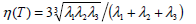
Three quality tests are carried out. The first test begins with the refinement of a single tetrahedron, namely a regular, a right or a poorly shaped one. Then the worst η-quality element from the eight sub-tetrahedra is determined. This element is refined again, and so on. The inner octaedron is always partitioned choosing the same diagonal (either the shortest or the longest) or choosing it randomly. No conformity of the resulting mesh is considered. Figure 2 depicts the mesh quality behavior as a function of refinement iterations for both shape measures.

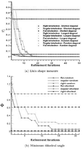
Figure 2: Quality metrics vs. refinement iterations for the first quality test

For these tetrahedra it is seen that the quality decrease produced by successive refinements is minimized if the shortest diagonal of the inner octahedron is always chosen. With this choice the quality of the mesh diminishes only at the first refinement iteration and then keeps constant. With the other choices the quality of the mesh tends to zero at each refinement iteration. Dihedral angles are plotted in radians.

The second test consists of refining 100,000 tetrahedra with the nodes coordinates randomly generated using a uniform distribution in the [0,1] interval. It is verified that neither the minimum dihedral angle nor the Liu's metric are always maximized if the shortest diagonal is used. For each tetrahedron, all diagonals of the inner octaedron are refined and the worst value of the quality criterion to be maximized is computed. Then the diagonal which maximizes the criterion is chosen. Both quality metric values corresponding to this diagonal (Opt) and the shortest diagonal (subscript Shortest) are considered. Only one refinement iteration is applied. The a posteriori analysis shows that in most cases (nearly 92 per cent of the samples for Liu's metric) using the shortest diagonal to refine the inner octaedron maximizes the quality criterion. Figure 3 depicts the maximum values for Liu's metric against those corresponding to the shortest diagonal. It can be seen that even when the shortest diagonal is not the best choice, the maximum relative loss of quality is 13 per cent. That is

(3)

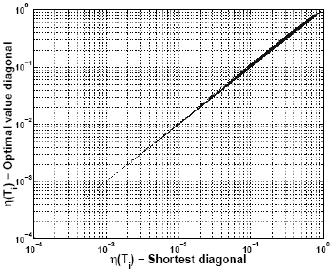
Figure 3: Liu's metric behavior for both the optimum value and shortest diagonal - 1e + 5 random sample tetrahedra.

Figure 3 also shows that for poorly shaped tetrahedra the relative loss of quality due to choosing the shortest diagonal is small. Finally, the computing time for the different strategies will be considered. If a strategy to maximize the quality criterion had to be used, all the three choices (one for each diagonal) should be taken into account. This could be too expensive for practical purposes, thus the shortest diagonal strategy is a good choice since it gives a final quality very close to the optimal one, with a much smaller computing effort.

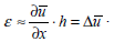
Lastly, in the third test, a sensitivity analysis to the initial tetrahedron shape is performed. Only one refinement iteration is done, always choosing the shortest diagonal. The starting tetrahedra are obtained moving one vertex of the regular tetrahedron on a plane parallel to its opposite face, as Fig. 4 shows. A non-linear dependency of the quality drop on the shape of the initial element can be observed in Fig. 5. The sensitivity is shown as a contour map of the ratio min(η(T¹))/η(T⁰), where the superscript indicates the number of refinement iteration to which the elements belong. This figure also shows that for some initial tetrahedral the quality does not diminish at all.

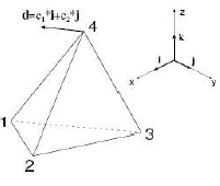
Figure 4: Starting tetrahedron.

Figure 5: Shape measure ratio min(η(T¹))/η(T⁰) contours for first refinement iteration - Shortest diagonal.

B. Refinement Algorithm

An adaptivity algorithm for unsteady problems must be computationally inexpensive, so that it can be applied every few time steps. To this end, it is decided both not to use transition elements to match zones with different levels of refinement and to use only one subdivision pattern for each type of element. As a consequence: a) the adapted mesh is non-conformal or has hanging nodes b) the 1-irregular node refinement constraint must be applied to ensure a gradual transition in the element size, c) mesh quality is not further degraded, d) there is no need to use compatibility rules for refinement / coarsening, and finally, e) the solution must be constrained on the hanging nodes. Figure 6 shows an example regarding to the 1-irregular node constraint if the shaded element is the one to be refined. Hanging nodes are marked with dots in the same figure. The 1-irregular node constraint says that no more than 1 hanging node should be shared amongst neighbouring elements through the common edge (2D and 3D) or face (3D) to which the node belongs. These kind of mesh refinemement was first proposed by Babuska and Rheinboldt (1978) for 2-D elements. In this work it is extended to the 3-D case. Some issues concerning to this kind of refinement are important: a) the problem solver has to be able to manage the constraint of the solution on the hanging nodes, b) the zone to be refined will be "wider" than the zone of interest in the solution field due to this solution constraint and c) some difficulties arise to visualize the results computed over meshes with irregular nodes, since contour lines are usually drawn element-wise for unstructured finite elements grids (Hannoun and Alexiades, 2007) and discontinuous contours appear.

Figure 6: 1-irregular node refinement constraint in 2- D.

To describe the refinement algorithm the following concepts about elements, faces and edges are introduced. It is said that an edge is active if not all the elements that share it are refined, otherwise it is inactive. The parent of an edge is the edge from which it derives by inserting a midpoint on the parent edge. The parent of a face is the face from which it derives by joining with edges the midpoints (and centre point in quads) that appear on the parent face. All the faces and edges that appear insid refined elements have no parents. Refined elements are always deactivated. Finally, every edge has two childs, every face has four childs and every element can have either 4 (2-D) or 8 (3-D) childs. These geometrical entities are organized in a hierarchical manner, so we say that an entity belongs to a low level of refinement if it has a higher hierarchy, and conversely.

Given a list of elements to be refined eles2ref, created either at the error estimate stage or prescribed by the user, the following algorithm is implemented:

1. Find the edges that belong to eles2ref. These edges are called edges2reftmp.

2. Find the edges in the set edges2reftmp that have not been refined yet and call them edges2ref.

3. Search the parent edges of the edges2ref. If some of them are still active, put them in a list ParentEdges2ref.

4. Find the elements to which these ParentEdges2ref belong and build a list eles2refNEW.

The same steps are taken for the faces. As a result, a new list of elements that should be refined at a lower refinement level is built within the actual iteration. Now, the refinement function is called with this list as argument. The recursivity ends when the list eles2refNEW in the actual iteration is empty. Then, the elements added to satisfy the 1-irregular criterion are refined from lower to higher levels until the original list of elements to be refined can be treated.

III. ADAPTIVITY STRATEGY

The unsteady strategy was developed based on the following concept: the adapted mesh is updated every n-time steps using a starting or base mesh, as the diagram on Fig. 7 depicts. For each one of these adaptivity steps (except for the first), some elements are marked to be refined, based on the error estimate chosen for the problem and the final solution computed at the previous adaptivity step. The elements to be refined are always selected at the maximum level of refinement. Since no higher level of refinement than the prescribed by the user is desired, a parents search algorithm should be used: if elements which do not belong to level 0 of refinement are selected, it is required to search for the parents of these elements in the data structure corresponding to this adaptivity step. The elements selected for refining are replaced by their parents and the process is repeated recursively until none of the elements in the list have parents (level 0). In this way, preliminary lists of elements to build each refinement level at the next adaptivity step are obtained. This process is represented by dashed lines in the diagram. Then, the next adaptivity step begins to be built.

Figure 7: Adaptivity strategy for unsteady problems.

Since the elements numbering scheme of the adapted meshes at the same refinement level changes from one adaptivity step to the next, the numbering of the elements in the preliminary list requiered to build that level needs to be updated. Once the list is updated, the corresponding level can be created. The updating and refinement processes are represented on the diagram by continuous and dotted lines, correspondingly. Finally, the problem solver is restarted using the most refined mesh. Only for the first adaptivity step, the problem solver is run a few time steps on the base mesh. Then, elements are marked and refined as many times as it is needed, based on the magnitude of the error estimates. The strategy does not consider coarsening of the base mesh and the adaptivity frequency is also constant through the whole run.

An initial state to restart the flow solver is computed as the linear interpolation of the solution on the last adapted mesh, at the nodes of the base mesh. The boundary conditions are also updated at every adaptivity step. To this end, geometrical entities of the mesh have a property flag attached to it. This flag is associated with a special property, such as a fixation, a periodic or a slip constraint, a geometrical or an elementary property or maybe an allowed combination of them. The properties are inherited from parents to childs at the refinement stage by inheritance of the flag, and updated lists of geometrical entities with that properties are built in a post-refinement stage within the adaptivity step.

IV. ERROR INDICATION

Since the exact solution of the problem is not known a priori, error estimates should be used to find which are the zones of the mesh that have to be refined. A great number of error estimate methods have been devised, most of them for elliptic problems. Mavriplis (1995) says that the choice of the right error indicator depends on multiple factors, such as the relative cost to compute the error estimate in regards to that of the rest of the adaptivity process, the affordable error estimate precision and the mathematical character of the equations. Heuristic gradient-based methods are frequently used in hyperbolic problems because they are computationally chipper, they let the zones to be refined be properly identified and because a more rigorous theory needs to be developed for hyperbolic equations. But success in using these kind of methods depends on the user's experience to choose the right combination of flow variables that better suit. For compressible flows, the gradient of the density and/or pressure fields are often used. An element is marked to be refined when the element-wise computed gradient multiplied by a measure of its size is greater than a prescribed tolerance value ε* for the error, that is

(4)

where

(5)

V. TEST CASE

To check the proper working of the unsteady strategy, the transient non-viscous supersonic flow at the starting of a bell-shaped rocket nozzle is solved. Also, to find out if there is a true efficiency gain, the same problem is solved over a fixed mesh finer than the base mesh used for the adaptive process and the clock time required by both runs is compared.

A. Problem Setup

While the axisymmetric flow equations are solved over an unstructured mesh of hexahedra, the adaptivity strategy is applied over the 2-D grid on the X-Z plane. Once the adapted mesh of quads is obtained, it is projected using the rotation matrix R(Φ). Figure 8 displays the problem setup. Only one layer of hexahedra is used in the circumferential direction Φ. Hexahedra nodes along the axis of symmetry are collapsed so that these elements turn into wedges. The nozzle area ratio is A/A*˜21.

Figure 8: Problem setup for the rocket nozzle.

Because of the axial symmetry of the flow, the following boundary conditions are considered

• Slip condition at the wall and along the axis of simmetry .

• Dynamic boundary conditions developed by Storti et al. (2008) are imposed at the exhaust section .

• Pressure and density are constants at the throat section . They linearly increase with time from the surrounding up to the stagnation values (?₀=0.47541 kg/m³, p₀=0.6MPa, T₀=4170K). Transient time for this condition is assumed to be t=5μsec.

• Axial flow at the throat section (V_xAD=0).

• There is no flux in the circumferential direction (V_Φ=0).

• Circumferential periodicity at every point of the domain.

On the other hand, the initial conditions in the whole domain take the following values (?_ini=0.0018$kg/m³, u_ini=0 m/s, p_ini=143 Pa, T_ini=262 K). The gas is considered to be air, and the isentropic coefficient value is γ=1.17.

B. Solving the Problem

The 3-D Euler equations are solved using the Advection-Diffusion module of the PETSc-FEM multi-physics FEM solver developed by Storti et al. (1999-2007), using 10 processors.

The Courant number for both the adaptive and non-adaptive simulations is Cou=2, except for the first time steps corresponding to the transient time at the throat conditions, when Cou=0.2. Selection of the elements to be refined is based on the magnitude of the element-wise computed velocity gradient . Velocity gradient is chosen because its scale range makes easier to apply the following criterion for selecting the elements to be refined

(6)

where constant c₁˜0.1 is adjusted beforehand for the whole run. Besides, the velocity gradient allows to capture the desired flow features with the mesh refinement.

One level of refinement is prescribed for the whole run and the adaptivity frequency is 5 time steps. This means that every 5 time steps the mesh is adapted to the last computed solution. It is considered that the problem has reached its stationary state for t_f=8.4e-4 sec, so this is the final time for the simulation. The base mesh for the adaptive simulation has 9330 elements and 9672 nodes while the mesh for the non-adaptive simulation has 11430 elements and 11842 nodes. Both of them have smaller size elements at the throat section. Figure 9 shows the size distribution of the elements for the base mesh, which is computed as the radius of the circumscircle of the quadrilateral elements on the X-Z plane.

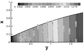
Figure 9: Element size distribution for the base mesh on the X - Z plane.

C. Results

The adaptive simulation requieres a few more time steps to reach the final time than the non-adaptive one, namely 2219 time steps for the latter and 2280 time steps for the former. The time steps number difference is due to the fact that, although the base mesh has fewer elements than the fixed, both the smaller size of the elements at the adapted zones and the CFL condition makes the time step smaller. Figure 10 shows that the size of the meshes in the adaptive simulation was never higher than the corresponding in the non-adaptive run.

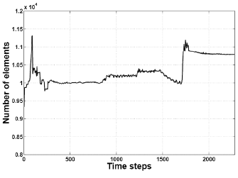
Figure 10: Number of elements behavior for the adaptive run.

The strange behavior in the number of elements is due both to the fact that the value changes with time and because of the non-uniform size distribution of the base mesh. Despite this difference in the number of time steps in favour of the non-adaptive simulation, the adaptive one is faster.

The axial velocity profiles are measured along the axis of symmetry at different time instants. They are shown at Fig. 11, where it can be seen that better resolution profiles correspond to the adaptive solution. The velocity increases behind the shock fronts which are traveling to the exit section of the nozzle. The local velocity shoot up immediately behind the secondary shock that appears in the non-adaptive profile at t=5e-4 sec. and t=6e-4sec. does not almost exists in the adaptive solution. It is worth to mention that all the variables of the flow were scaled due to numerical reasons. Therefore the velocity scale should be multiplied by V_ref=1215.16 m/sec to get the actual velocity values in the figures.

Figure 11: Comparison of axial velocity profiles along the axis of symmetry.

Velocity contours are compared for the same time instant at Fig. 12. Better resolution of the shock fronts is apparent for the adaptive solution. Although along the axis of symmetry the velocity contours are rather similar, evident differences exists close to the nozzle wall. Finally, details of the adapted meshes at the shock fronts are presented for two time instants in Fig. 13. It can be seen that at t=3.5 e-4 sec. the velocity gradient at the secondary shock location was not still big enough as to trigger there the refinement of the mesh.

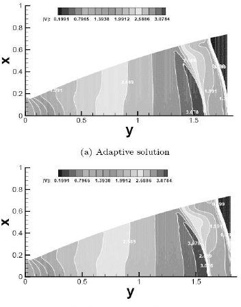
Figure 12: Velocity contours comparison at t = 6e- 4sec.

Figure 13: Adaptively refined meshes at the shock front locations.

V. CONCLUSIONS

A strategy to adaptively solve unsteady problems over unstructured finite element meshes has been presented. The numerical quality tests show that there exists a partition procedure for tetrahedral elements which keeps bounded the decrease of the mesh quality. The refinement algorithm to apply this procedure has been described. It is considered that efficiency and low computational costs are its main advantages while the management of the hanging nodes may cause some problems for visualizing the results. The first test case over an unstructured mesh of hexahedra proves that better use of computational resources can be achieved using the adaptive solver. Both a better resolution and a shorter simulation time give support to this conclusion. The capability of the adaptive code to handle different type of boundary conditions has also been tested. Future work includes applying the unsteady strategy over unstructured meshes of tetrahedra.

ACKNOWLEDGMENT
This work has received financial support from Consejo Nacional de Investigaciones Científicas y Técnicas (CONICET, Argentina, grant PIP 5271/05), Universidad Nacional del Litoral (UNL, Argentina, grant CAI+D 2005-10-64) and Agencia Nacional de Promoción Cientíca y Tecnológica (ANPCyT, Argentina, grants PICT 12-14573/2003, PME 209/2003, PICT-1506/2006). Authors made extensive use of freely distributed software from the GNU Project and others, as Fedora GNU/Linux~OS, MPI, PETSc, the GCC compiler collection, Octave, Open-DX, among many others. Also, many ideas from these packages have been inspirational to them.

REFERENCES

1. Babuska, I. and W.C. Rheinboldt, "Error estimates for adaptive finite element computations," SIAM J. Numer. Anal., 15, 736-754 (1978).         [ Links ]

2. Hannoun, N. and V. Alexiades, "Issues in adaptive mesh refinement implementation," Electronic Journal of Differential Equations, 15, 141-151 (2007).         [ Links ]

3. Knupp, P.M., "Algebraic mesh quality metrics," SIAM Journal of Scientific Computing, 23, 193-218 (2001).         [ Links ]

4. Liu, A. and B. Joe, "On the shape of tetrahedra from bisection," Mathematics of Computation, 63, 141-154 (1994).         [ Links ]

5. Mavriplis, D.J., "Unstructured mesh generation and adaptivity," Report 95-26, ICASE - NASA Langley Research Centre, April (1995).         [ Links ]

6. Ríos Rodríguez G.A., E.J. López, N.M Nigro and M. Storti, Refinamiento adaptativo homogéneo de mallas aplicable a problemas bi- y tridimensionales (2005).         [ Links ]

7. Storti, M.A., N. Nigro, R. Paz, L. Dalcín and E. López. PETSc-FEM, A General Purpose, Parallel, Multi-Physics FEM Program. CIMEC-CONICET-UNL, (1999-2007).         [ Links ]

8. Storti, M.A., N.M. Nigro, R.R. Paz and L.D. Dalcín, "Dynamic boundary conditions in computational fluid dynamics," Computer Methods in Applied Mechanics and Engineering, 197, 1219-1232 (2008).         [ Links ]

Received: April 8, 2008.
Accepted: June 27, 2008.
Recommended by Subject Editor: Eduardo Dvorkin.