ARTICLES

Change detection in time series using the maximal overlap discrete wavelet transform

V. Alarcon-Aquino^† and J. A. Barria^‡

^† Department of Computing, Electronics, and Mechatronics, Universidad de las Americas Puebla CP 72820, MEXICO
vicente.alarcon@udlap.mx
^‡ Department of Electrical and Electronic Engineering, Imperial College London, SW7 3DU, UK

Abstract - The problem of change detection of time series with abrupt and smooth changes in the spectral characteristics is addressed. We first review the main characteristics of the discrete wavelet transform and the maximal overlap discrete wavelet transform. An algorithm for sequential change detection in time series is then reported based on the maximal overlap discrete wavelet transform and Bayesian analysis. The wavelet-based algorithm checks the wavelet coefficients across resolution levels and locates smooth and abrupt changes in the spectral characteristics in the given time series by using the wavelet coefficients at these levels. Simulation results demonstrate the good detection properties of the proposed algorithm when compared with previous reported algorithms, and also indicate that the quadratic spline and least-asymmetric wavelets have less amount of shift in position after wavelet decomposition and therefore an alignment of events to be detected in a multi-resolution analysis with respect to the original time series is obtained.

Keywords - Wavelets; Wavelet Transforms; Change Detection; Time Series.

I. INTRODUCTION

During the past decade, wavelet transforms have emerged as an important mathematical tool for the analysis of time series (see e.g. Khalil Khalil and Duchene, 1999; Percival and Walden, 2000; Bakshi, 1999; Kobayashi, 2001; Alarcon-Aquino, 2003; Salam et al., 2008) and have found applications in anomaly detection, time series prediction, image processing, and noise reduction (see e.g., Khalil Khalil and Duchene, 1999; Kobayashi, 2001; Alarcon-Aquino, 2003; Alarcon-Aquino and Barria, 2002; Alarcon-Aquino and Barria, 2006; Alarcon-Aquino and Barria, 2001; Tseng et al., 2006). In particular, the wavelet transform provides an interesting framework for the analysis of non-stationary signals, and it is an alternative to the classical classical Short Time Fourier Transform (STFT). The STFT applies a moving window over the data to determine the localized spectra. A drawback of the STFT is that the time-frequency window is fixed whereby the window cannot adapt to the characteristics of the signal at a certain point (Mallat, 1999; Daubechies, 1992). The wavelet transform uses small window widths at higher frequencies and large window widths at low frequencies. That is, it is well-suited for signals where high frequency signal components have shorter duration than low frequency signal components (Mallat, 1999). This is due to the so-called constant relative bandwidth frequency analysis (Percival and Walden, 2000). The wavelet transform applies bases which are either finite support or die quickly after a finite interval. These bases have better characteristics to "zoom-in" on very short-lived high frequency phenomena such as transients in signals. Further details on wavelets and wavelet transforms can be found in (Mallat, 1999; Daubechies, 1992; Percival and Walden, 2000).

The signals encountered in practice are usually random and non-stationary. The modeling of these signals and specifically quasi-stationary signals have been a continuing subject of research for many years (see e.g., Khalil and Duchene, 1999; Baseville and Nikiforov, 1993; Percival and Walden, 2000; Bakshi, 1999; Tseng et al., 2006; Salam et al., 2008). Quasi-stationary signals are characterized by abrupt changes in the statistical properties at unknown instants and stationary behavior in between those instants. These instants are called segment boundaries. To perform an analysis of these stationary segments we may use parametric models. Studies on adaptive sequential segmentation include a sequential generalized likelihood ratio (GLR) test (Appel and Brandt, 1983; Salam et al., 2008), the divergence test (Basseville and Nikiforov, 1993; Salam et al., 2008), Bayesian approaches (Basseville and Nikiforov, 1993), and genetic algorithms (Tseng et al., 2006) The work reported in this paper investigates the viability and usability of discrete wavelet transforms in adaptive sequential segmentation of non-stationary signals. The proposed algorithm checks the wavelet coefficients across resolution levels and locates smooth and abrupt changes in the spectral characteristics of the given time series by using the wavelet coefficients at these levels, and it is compared with two well-known adaptive segmentation algorithms : the Brandt's GLR test and the divergence test (Salam et al., 2008). The rest of the paper is organized as follows. An overview of the discrete wavelet transform and the maximal overlap discrete wavelet transform is presented in Section II. In Section III, the proposed wavelet-based detection algorithm is described and the unknown variance of the wavelet coefficients is eliminated by marginalization (Gustafsson, 1996) using the Inverse Wishart as Prior. Other priors are assessed in Alarcon-Aquino (2003). Section IV provides some representative examples using synthetic data, in which the proposed approach and the classical approaches in segmentation of non-stationary signals are compared. A discussion of a wavelet choice is also addressed. Finally, Section V summarizes the conclusions drawn from previous sections.

II. REVIEW OF WAVELET TRANSFORMS

Wavelet transforms involve representing a general function in terms of simple, fixed building blocks at different scales and positions. These building blocks are generated from a single fixed function called mother wavelet by translation and dilation operations. Thus, wavelet transforms are capable of "zooming-in" on short-lived high frequency phenomena, and "zooming-out" on long-lived low frequency phenomena. The continuous wavelet transform considers a family (Mallat, 1999)

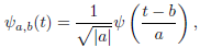(1)

where ∈ ℜ⁺, ∈ ℜ, with ≠ 0, and ψ(·) satisfies the admissibility condition. For discrete wavelets the scale (or dilation) and translation parameters in Eq. (1) are chosen such that at level j the wavelet is times the width of ψ(t). That is, the scale parameter 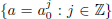and the translation parameter 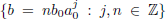. This family of wavelets is thus given by

(2)

A. Orthonormal bases and Multi-resolution Analysis

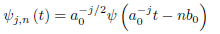
The mother wavelet function ψ(t), scaling and translation parameters are specifically chosen such that ψ_j,n(t) constitute orthonormal bases for L²(ℜ) (Mallat, 1999; Daubechies, 1992). To form orthonormal bases with good time-frequency localization properties, the time-scale parameters (, ) are sampled on a so-called dyadic grid in the time-scale plane, namely, = 2 and = 1, (Mallat, 1999; Percival and Walden, 2000). Thus, from Eq. (2) substituting these values, we have a family of orthonormal bases,

(3)

The orthonormal wavelet transform is thus given by (Mallat, 1999)

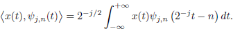(4)

A formal approach to constructing orthonormal bases is provided by multi-resolution analysis (MRA). The idea of MRA is to write a function x(t) as a limit of successive approximations, each of which is a smoother version of x(t). The successive approximations thus correspond to different resolutions. Multiresolution analysis is defined as sequences of closed subspaces{V_j ⊂ L²(ℜ): j ∈ } with the following properties (Mallat, 1999):

(i) ...V₂ ⊂ V₁ ⊂ V₀ ⊂ V₋₁ ⊂ V₋₂ ⊂ ... ⊂ L²(ℜ) (i.e., V_j ⊂ V_j−1);
(ii) V_j = {0}, and, = L²(ℜ);
(iii) ∀j ∈ , x(t) ∈ V_j ⇔ x(2t) ∈ V_j−1;
(iv) ∀k ∈ , x(t) ∈ V₀ ⇒ x(t − n) ∈ V₀;
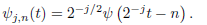
(v) There exists a function φ(t) ∈ V₀ such that {φ_j,n(t) = 2^−j/2φ(2^−jt − n): j, n ∈ } satisfies Eq. (4) and forms an orthonormal basis of V₀.

An explanation of these properties follows. Property (i) denotes the successive subspaces that are used to represent the different resolutions or scales, while property (ii) guarantees the completeness of these subspaces and ensures that lim_j→−∞ x_j(t)= x(t). Property (iii) denotes that V_j−1 consists of all re-scaled versions of V_j, while property (iv) means that any translated version of a function belongs to the same space as the original. Finally, in property (v), the function φ(·) is called the scaling function in the multi-resolution analysis (Daubechies, 1992; Mallat, 1999).

B. Discrete Wavelet Transform: Decomposition and Reconstruction

Since the idea of multi-resolution analysis is to write a signal x(t) as a limit of successive approximations, the differences between two successive smooth approximations at resolution 2^j−1 and 2^j give the detail signal at resolution 2^j. In other words, one has an initial resolution J, any signal x(t) ∈ L²(ℜ) can then be expressed as (Mallat, 1999; Daubechies, 1992):

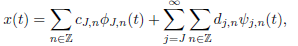(5)

where (φ(t)) denotes the scaling function and the details or wavelet coefficients {d_j,n} are defined by

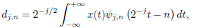(6)

while the approximations or scaling coefficients {c_j,n} are defined by

(7)

Equations (6) and (7) express that a signal x(t) is decomposed in details {d_j,n} and approximations {c_j,n} to form a multi-resolution analysis of the signal (Mallat, 1999). An attractive property of wavelets is that there exists a recursive relationship between scaling ({c_j,n}) and wavelet coefficients ({d_j,n}) at successive levels of resolution. That is, by using Eq. (7) and the dilation equation (Daubechies, 1992) yields

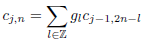(8)

(9)

where (g_l) represents the coefficients of a low-pass filter (or scaling filter) and (h_l) denotes the coefficients of a band-pass filter (or wavelet filter). Note that the sequences {c_j,n} and {d_j,n} are generated by downsampling by a factor of two the output of the corresponding filters.

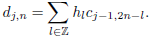
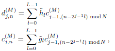
Equations (8) and (9) denote approximation and details coefficients respectively at level of resolution j and these are obtained from approximation coefficients at finer level of resolution j −1. In the opposite direction, approximation coefficients at level of resolution j − 1 are computed from scaling and wavelet coefficients at the coarser level of resolution j according to

(10)

The sequence {c_j−1,n} is generated by up-sampling the output of the corresponding filters. This operation is achieved by inserting one zero every two samples. Equations (8)-(10) can be computed by a pyramid algorithm (Mallat, 1999) called discrete wavelet transform (DWT). The DWT has some limitations. For example, it requires the sample size N to be an integer multiple of 2^J and the number {N_j} of scaling and wavelet coefficients at each level of resolution j decreases by a factor of two, due to the decimation process that needs to be applied at the output of the corresponding filters. This can introduce ambiguities in the time domain. The down-sampling process can be avoided by using the maximal overlap discrete wavelet transform (MODWT) (Percival and Walden, 2000), which is also known as the undecimated discrete wavelet transform (Mallat, 1999). The MODWT may be computed for an arbitrary length time series. Note, however, that the MODWT requires (N log₂ N) multiplications, whereas the DWT can be computed in (N) multiplications. There is, thus, an increase in computational complexity when using the MODWT. However, its computational burden is the same as the widely used fast Fourier transform algorithm and hence quite acceptable (Percival and Walden, 2000).

C. The Maximal Overlap Discrete Wavelet Transform

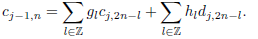
In this section we introduce the maximal overlap discrete wavelet transform (MODWT). To build the MODWT a rescaling of the defining filters is required to conserve energy, that is, and , so that = 1/2, and therefore the filters are still quadrature mirror filters (QMFs). The wavelet filter must satisfy the following properties (Percival and Walden, 2000):

(11)

(12)

for all non zero integers r, where (L) denotes the length of the wavelet filter. The scaling filter is also required to satisfy Eq. (12) and = 1. Now let be the time series, the MODWT pyramid algorithm generates the wavelet coefficients and the scaling coefficients from , where (M) stands for MODWT. That is, with nonzero coefficients divided by , the convolutions can be written as follows (Percival and Walden, 2000):

(13)

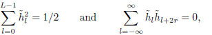
where n = 0, 1,...,N − 1, and (N) denotes the length of the time series to be analyzed. Equation (13) can also be formulated as circular filter operations of the original time series {x_n} using the filters 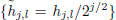and 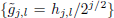(see Fig. 1), namely,

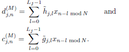(14)

Figure 1: Wavelet decomposition of MODWT. The wavelet coefficients and scaling coefficients are computed by cascading convolutions with filter .

The original signal can be recovered from and using the inverse pyramid algorithm (Percival and Walden, 2000),

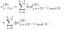(15)

where n = 0, 1,...,N − 1. Note that for each level of resolution j (or scale), the mean of wavelet coefficients for the MODWT is equal to zero (see Eq. (14)), viz.

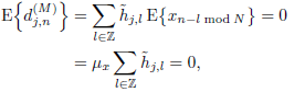(16)

where µ_x is the mean of the analyzed time series, and by using the fact that = 0 (see Eq. (11)), the result follows (Alarcon-Aquino, 2003). This property is used normally in wavelet-based detection algorithms for detecting sudden jumps in the mean (see e.g., Alarcon-Aquino, 2003; Alarcon-Aquino and Barria, 2001).

III. PROPOSED CHANGE DETECTION ALGORITHM

In this section, an on-line change detection algorithm based on wavelets is proposed for segmentation of time series based on the MODWT and Bayesian analysis. The wavelet-based detection algorithm checks the wavelet coefficients across resolution levels, and detects smooth and abrupt changes in variance and frequency in the given time series by using the wavelet coefficients at these levels (Alarcon-Aquino, 2003). This method has the advantage of adapting locally to the features of the signal. By contrast, standard segmentation algorithms (see e.g., Gustafsson, 1996; Appel and Brandt, 1983; Basseville and Nikiforov, 1993; Salam et al., 2008) analyse the given time series at fixed resolution in time or frequency. In the wavelet-based algorithm, we consider the unknown variance of the wavelet coefficients as a stochastic nuisance parameter. Marginalization is then used to eliminate this nuisance parameter in the wavelet domain using the inverse Wishart distribution (scalar case). The wavelet-based detection algorithm is evaluated using synthetic data and compared with standard segmentation algorithms.

A. Problem Formulation and Assumptions

Let the time series xn be modeled by

(17)

where denotes the regression vector, θ_n denotes the unknown parameters of the signal model and is the unknown changing variance. The likelihood for data = x₁,x₂,...,x_N given the parameters θ_n and is thus denoted by . The vector Θ = {θ_n,} is the parameter of interest. The vector is Θ = Θ_a until the unknown time t₀ and from t₀ + 1 the vector becomes Θ = Θ_b. Therefore, the discrete time model (Θ) with changes in the parameters is given by

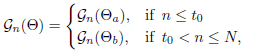(18)

where (Θ_a) denotes the normal operation mode of the model and (Θ_b) is the mode with changes either in θ_n or in . Note that since multi-scale decomposition of a signal is equivalent to a band-pass filtering and modifications in the process will mainly lead to variance changes (see e.g., Khalil and Duchene, 1999), the approach studied in this paper is free of model selection parameters and hence the problem is reduced to the estimation of unknown changing variance. In order to determine whether a change has occurred at time t₀, the adaptive learning wavelet-based algorithm uses a sliding window approach. This approach considers two windows; a test window and a reference (or learning) window, from which two models are derived (see Fig. 2). These two models are then used for the waveletbased detection algorithm to perform the sequential decision process. In each time interval or window, the wavelet coefficients are modeled as Gaussian stationary process 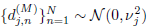, for j = 1, 2,...,J, where represents the unknown changing variance of wavelet coefficients at each scale j. 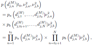The test window based on data 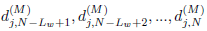of length L_w is compared to a growing reference window based on all previous data or larger L_w, to determine whether both models are generated by the same or different distributions. If no change point is detected, then the arrival of new data to a test window of length L_w causes the oldest datum to move into the learning window. Otherwise, the wavelet-based segmentation algorithm performs a decision function. Further details on sliding window approaches can be found in (Basseville and Nikiforrov, 1993). The likelihood for data can be computed as a product of the likelihoods before and after change. That is, the likelihood of the change point having taken place at t₀ = N − L_w, where L_w is the length of a sliding test window, is given by (Alarcon-Aquino, 2003)

(19)

for j = 1, 2,...,J.

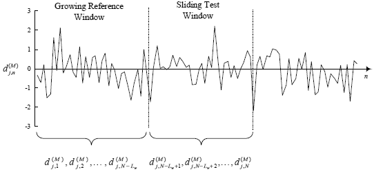
Figure 2: Reference and sliding test windows for online detection of changes.

The unknown changing variances for n ≤ t₀ and for t₀ < n ≤ N are considered nuisance parameters, and are removed in the wavelet domain after integrating with respect to a prior distribution. Thus, based on the model described by Eq. (18), the following hypotheses are compared:

and the alternative hypothesis:

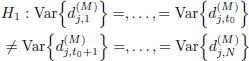
where j = 1, 2,...,J and t₀ = N − L_w denotes an unknown change point. The hypothesis H₁ occurs when there is a change on the variance of wavelet coefficients between the reference and the sliding test windows. Otherwise, the null hypothesis H₀ occurs.

At the core of our derivations are the so-called nuisance parameters, these nuisance parameters can be estimated or marginalized. The usual likelihood-ratio testing procedure involves computing the maximum likelihood estimates of the unknown nuisance parameters (see e.g., Basseville and Nikiforov, 1993). In contrast, the concept of marginalization is to assign a prior distribution to the unknown nuisance parameter and eliminate it from the analysis (see e.g., Gustafsson, 1996). This means that the likelihoods are marginal in the sense that they are obtained after integrating out the nuisance parameters. The unknown change points are then estimated by comparing the posterior probabilities computed using Bayes' theorem (Bernardo and Smith, 1994). The posterior probability associated with H₀ can be obtained by inserting p(H₀) and integrating with respect to a prior distribution of the nuisance parameter , namely,

(20)

where denotes the unknown variance of wavelet coefficients at scale j, t₀ is an unknown change point and is the prior to be considered, i.e., the inverse Wishart distribution (scalar case). Similarly, the second hypothesis checks H₁ whether a change has occurred on the variance of wavelet coefficients, viz.

(21)

where t₀ = N − L_w is an unknown change point. The prior probabilities associated with the hypotheses are p(H₀) and p(H₁) with p(H₀)+ p(H₁) = 1. Asaresult, p(H₀) = π_p for π_p ∈ (0, 1) and p(H₁) = 1 − π_p since H₁ is the complement of a simple hypothesis H₀. Equations (20) and (21) can be solved by using . This result is easily obtained by using the change-of-variable rule (Bernardo and Smith, 1994). The unknown change points are then estimated by comparing the posterior probabilities computed using Bayes' theorem. In order to obtain the posterior probability associated with the hypothesis H₀, consider the inverse Wishart distribution W(m, S) as prior on the variance of wavelet coefficients . Using Eq. (20), the posterior probability associated with the hypothesis H₀, using the inverse Wishart distribution as prior on the variance of wavelet coefficients, is given by

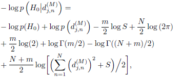(22)

for j = 1, 2,...J.

where m and S are the hyper-parameters of the inverse Wishart distribution (see Bernardo and Smith, 1994) used for . Using Stirling's formula, Γ ( + 1) ≈ (Bernardo and Smith, 1994), on the gamma function Γ (·), Eq. (22) can be approximated as:

(23)

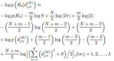
The second hypothesis H₁ checks whether a change has occurred on the variance of wavelet coefficients. Using Eq. (21) the posterior probability associated with the hypothesis H₁, using the inverse Wishart distribution as prior on the variance of wavelet coefficients, is given by

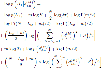(24)

for j = 1, 2,...J.

where m and S are the hyper-parameters of the inverse Wishart distribution used for . Using Stirling's formula on the gamma function Γ (·), Eq. (24) can also be simplified as Eq. (23). Change points are then estimated by comparing the posterior probabilities.

IV. SIMULATION RESULTS

In this section, the simulated data are generated by switching auto-regressive (AR) filters with time invariant parameters, which are driven by the same Gaussian white noise source (Appel and Brandt, 1983). This set of data series simulates different kinds of changes, such as abrupt and smooth changes in the AR parameters. The AR vector parameter changes from (−0.5, 0.5) to (−0.9, 0.9) at N = 100 from (−0.9, 0.9) to (−0.6, 0.6) at N = 250, and from (−0.6, 0.6) to (−0.67, 0.67) at N = 500. A ramp behavior from N = 800 to N = 899 is also included, which simulates a smooth change in the signal. In this example, the in-verse Wishart prior and three wavelets are assessed: a quadratic spline wavelet, Daubechies' family wavelets, and the Haar wavelet (Mallat, 1999; Daubechies, 1992; Percival and Walden, 2000). The sliding test window is set at L_w = 75. Note that the sliding test window (L_w) may be chosen based on the desired delay for detection. That is, a possible starting value is the specified mean delay for detection.

In general, the following criteria may be used when selecting the value of the sliding test window, the length of the segment to be detected and the detection delay. Further details can be found in (Alarcon-Aquino, 2003).

A. Wavelet Choice

The selection of the wavelet must be related to the common features of the events present in real signals. That is, the wavelet should be well adapted to the events to be analyzed (Alarcon-Aquino, 2003). Different wavelet families¹ have a trade-off between the degree of symmetry (i.e., linear phase characteristics of wavelets) and the degree to which ideal high-pass filters are approximated (Percival and Walden, 2000). The degree of symmetry in a wavelet is important in reducing the phase shift of features during the wavelet decomposition. If the phase shift is large, it can lead to distortions in the location of features in the transform coefficients. The degree to which ideal high-pass filters are approximated is also important since, ideally, the wavelet filter should resemble a high-pass (j = 1) or band-pass (j > 1) filter, while the scaling filter should resemble a low-pass filter. In this section, these issues are shortly discussed for the following wavelets: the Haar wavelet, Daubechies' family wavelets and a quadratic spline wavelet.

The Haar wavelet−The simplest wavelet basis for L²(ℜ) is the Haar basis (Daubechies, 1992). The Haar wavelet filter is of length L = 2. The scaling filter is the two element vector g₀ = g₁ = and the wavelet filters are h₀ = and h₁ = − . The Haar wavelet has compact support; however, it has just one vanishing moment and is piece-wise constant. Furthermore, the resulting wavelet basis functions have the significant additional disadvantage of being discontinuous, which renders them unsuitable as basis functions for classes of smoother functions. Figure 3 shows the squared magnitude responses |H_j (f)|² (solid line) and |G_j (f)|² (dash-dotted line) for the Haar wavelet and scaling filters, respectively. This figure shows that the Haar wavelet filter appears to be a poor approximation to an ideal band-pass filter for all scales shown. That is, the Haar wavelet filter shows significant leakage (cross-hatched areas) from both higher and lower frequencies (Percival and Walden, 2000).

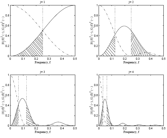
Figure 3: Squared magnitude responses for the Haar wavelet (solid line) and scaling (dash-dotted line) filters at scales j = 1, 2, 3, 4.The vertical dotted lines denote the frequency bands for an ideal bandpass filter.

Daubechies wavelets−To overcome the disadvantage of the Haar wavelet, Daubechies (Daubechies, 1992) has developed a theory for obtaining higher order mother wavelet filters with compact support and has also identified two set of filters, namely, the extremal phase (D) and the least asymmetric (LA) or symmlets. These filters have even lengths L (between 2 and 20); however, they are identified not by the length L but by the number of vanishing moments, v = L/2. As the number of vanishing moments increases, the wavelet filter becomes longer and its approximation to an ideal high-pass filter improves. That is, a lesser amount of leakage is obtained, which is caused by the non-ideal filter shape (see e.g., Alarcon-Aquino, 2003). The order of the filter is equal to the number of vanishing moments and, for the case, of Daubechies filters, it is half the length of the filter. Note that for v = 1, the Daubechies wavelet filter is equivalent to the Haar wavelet filter.

Quadratic spline wavelet - The quadratic spline wavelet has a small compact support, one vanishing moment, and it is the first derivative of the cubic spline function. That is, linear phase filters such as the quadratic spline wavelet and least asymmetric wavelets have less amount of leakage. This characteristic reduces the amount of shift in position after wavelet decomposition and therefore an alignment of events in a multi-resolution analysis with respect to the original time series is obtained (see e.g., Alarcon-Aquino, 2003).

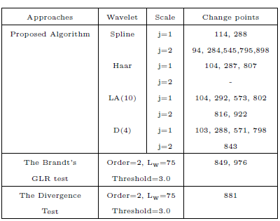
Table 1 illustrates the estimated change points of the proposed wavelet-based change detection algorithm, the Brandt's GLR test and the divergence test(Salam et a.., 2008). The change points for the waveletbased change detection algorithm are estimated by comparing the posterior probabilities computed using Bayes' theorem. The table shows that proposed wavelet-based change detection algorithm using the quadratic spline wavelet and the LA(10) wavelet is able to detect and locate the boundary of each segment. For the quadratic spline wavelet the algorithm detects the abrupt changes at N = 114, 288 at j = 1 and at N = 94, 284 with scale j = 2. Smooth changes are also detected with the quadratic spline wavelet at N = 545, 795, 898 with scale j = 2. Note that the best performance is achieved with the quadratic spline wavelet and the LA(10) wavelet. This is expected since the quadratic spline wavelet and the LA(10) have linear phase. This characteristic allows alignment of events with respect to the original time series after wavelet decomposition (Percival and Walden, 2000). The Haar wavelet does not give good results for approximated smooth changes mainly because it has only one vanishing moment and is piece-wise constant (Mallat, 1999; Daubechies, 1992). Note that the Brandt's GLR test and the divergence test are unable to identify the subtle changes at N = 500 and in some cases abrupt changes at N = 100, 250. Other performance comparisons have been presented in (Khalil and Duchene, 1999; Tseng et al., 2006) where it is also shown that multi-scale approaches outperform autoregressive approaches.

Table 1: Estimated change points for the proposed wavelet-based change detection algorithm, Brandt's GLR test (Appel and Brandt, 1983; Salam et al., 2008) and the divergence test (Basseville and Nikiforov, 1993; Salam et al., 2008).

The selection of the number of scales depends primarily on the time series at hand. Since the scale choice depends on the wavelet itself, the number of scales is chosen according to the overall energy displayed at each scale (see e.g., Alarcon-Aquino, 2003).

V. CONCLUSIONS

In this paper a sequential change detection algorithm using the maximal overlap discrete wavelet transform and Bayesian analysis has been reported.The waveletbased detection algorithm was able to identify smooth and abrupt changes in the variance by using the wavelet coefficients at these levels. The unknown variance of the wavelet coefficients was considered as a stochastic nuisance parameter. Marginalization was then used to eliminate this nuisance parameter using the Inverse Wishart distribution as prior. A discussion was also carried out on different wavelet families that have a trade-off between the degree of symmetry and the degree to which ideal high-pass filters are approximated. It was found that linear phase filters such as the quadratic spline wavelet and leastasymmetric wavelets have less amount of leakage. This characteristic reduces the amount of shift in position after wavelet decomposition. In general, the results show that the best performance was obtained with the quadratic spline wavelet and the LA(10) wavelet. This is to be expected due to the fact that these wavelets have linear phase and there is therefore an alignment between the original time series and the wavelet coefficients. The wavelet-based detection algorithm reported in this paper may be applied in segmentation of speech signals, traffic analysis for network intrusion detection, detection of vibrations in mechanical systems, harmonic detection, and several other applications in medicine.

---

¹A wavelet family consists of all wavelet basis vectors for all dilations and translations derived from a single mother wavelet ψ(t).

REFERENCES

1. Alarcon-Aquino, V., Anomaly Detection and Prediction in Communication Networks Using Wavelet Transforms, PhD Thesis, Imperial College London, University of London (2003).         [ Links ]

2. Alarcon-Aquino, V. and J.A. Barria, "Anomaly Detection in Communication Networks Using Wavelets," IEE Proceedings -Communications, 148, 355-362 (2001).         [ Links ]

3. Alarcon-Aquino, V. and J.A. Barria, "Multi-Sensor Fusion System Using Wavelet Based Detection Algorithm Applied to Network Monitoring,"Proceedings of London Communication Symposium, 361-364 (2002).         [ Links ]

4. Alarcon-Aquino, V. and J.A. Barria, "Multiresolution FIR Neural Network Based Learning Algorithm Applied to Network Traffic Prediction," IEEE Transactions on Systems, Man and Cybernetics Part C: Applications and Review, 36, 208-220 (2006).         [ Links ]

5. Appel, U. and A.V. Brandt, "Adaptive Sequential Segmentation of Piecewise Stationary Time Series", Information Sciences, 29, 27-56 (1983).         [ Links ]

6. Bakshi, B.R., "Multiscale Analysis and Modelling Using Wavelets," Journal of Chemometrics, 13, 415-434 (1999).         [ Links ]

7. Bernardo, J.M. and A.F.M. Smith, Bayesian Theory, NY Wiley (1994)        [ Links ]

8. Basseville, M. and I.V. Nikiforov, Detection of Abrupt Changes: Theory and Application. Information and System Science Series. Englewood Cliffs, NJ: Prentice-Hall (1993).         [ Links ]

9. Daubechies, I. Ten Lectures on Wavelets, New York: SIAM (1992).         [ Links ]

10. Gustafsson, F., "The Marginalised Likelihood Ratio Test for Detecting Abrupt Changes," IEEE Transactions on Automatic Control, 41, 66-78 (1996).         [ Links ]

11. Khalil, M. and J. Duchene, "Detection and Classification of Multiple Events in Piecewise Stationary Signal: Comparison between autoregressive and multiscale approaches," Signal Processing, 75, 239-251 (1999).         [ Links ]

12. Kobayashi, M.,"Wavelet Analysis and Their Applications in Industry," Nonlinear Analysis, 47, 1749-1760 (2001).         [ Links ]

13. Mallat, S. A Wavelet Tour of Signal Processing, Academic Press (1999).         [ Links ]

14. Percival, D.B. and A.T. Walden, Wavelet Methods for Time Series Analysis. Cambridge University Press (2000)        [ Links ]

15. Salam, M-S., D. Mohaman and S-H Salleh, "Segmentation of Malay Syllables in Connected Digit Speech Using Statistical Approach," International Journal of Computer Science and Security, 2, 23-33 (2008).         [ Links ]

16. Tseng,V.S., C.H. Chen, C-H Chen and T-P Hong., "Segmentation of Time Series by the Clustering and Genetic Algorithms," in Proceedings of the Sixth International Conference on Data Mining-Workshops ICDMW06 (2006).         [ Links ]

Received: March 14, 2008.
Accepted: August 21, 2008.
Recommended by Subject Editor: Jorge Solsona.