Relative error control in quantization based integration

E. Kofman

CIFASIS-CONICET. Laboratorio de Sistemas Dinámicos FCEIA -UNR. Riobamba 245 bis -(2000) Rosario.

Abstract — This paper introduces a method to achieve relative error control in Quantized State System (QSS) methods. Based on the use of logarithmic quantization, the proposed methodology solves the problem of quantum selection.

Keywords — Quantization Based Integration. Continuous System Simulation.

I. INTRODUCTION

Numerical integration of ordinary differential equations (ODEs) is a topic of permanent research and development. Based on classic methods like Euler, Runge-Kutta and Adams and impulsed with the development of modern and fast computers, several variable-step and implicit ODE solver methods were introduced (Hairer et al., 1993; Hairer and Wanner, 1991; Cellier and Kofman, 2006).

Simultaneously, different software simulation tools implementing those modern methods have been developed. Matlab/Simulink (Shampine and Reichelt, 1997) and Dymola (Elmqvist et al., 1995) can be mentioned among the most popular and efficient general purpose ODE simulation packages.

In spite of the several differences between the mentioned ODE solvers, all of them share a property: they are based on time discretization. This is, they give a solution obtained from a difference equation system, i.e. a discrete-time model.

A completely different approach started to develop since the end of the 90's, where time discretization is replaced by state variables quantization. As a result, the simulation models are not discrete time but discrete event systems. The origin of this idea can be found in the definition of Quantized Systems (Zeigler et al., 2000).

This idea was then reformulated with the addition of hysteresis -to avoid the appearance of infinitely fast oscillations- and formalized as the Quantized State Systems (QSS) method for ODE integration in (Kofman and Junco, 2001). This was followed by the definition of the second order QSS2 method (Kofman, 2002), the third order QSS3 method (Kofman, 2006), a first order Backward QSS method (BQSS) for stiff systems (Migoni et al., 2007), and a first order Centered QSS for marginally stable systems.

The QSS-methods show some important advantages with respect to classic discrete time methods in the integration of discontinuous ODEs (Kofman, 2004), sparsity exploitation (Kofman, 2002), explicit integration of stiff and marginally stable systems (Migoni et al., 2007), absolute stability, and the existence of a global error bound (Cellier and Kofman, 2006).

One of the major drawbacks of the QSS methods is the need of choosing a quantization parameter (called quantum) for each state variable, as the efficiency and accuracy of the simulation depends strongly on this choice. The problem is also related to the fact that the methods intrinsically control the absolute error instead of the relative error as classic variable step methods do.

This work shows that the use of time varying quantization, proportional to the magnitude of each state variable (i.e., logarithmic quantization), leads to an intrinsic relative error control in the QSS methods. Moreover, it will be shown that the relative error is approximately proportional to the constant factor that relates the quantum with the state magnitude. This property will permit selecting directly the relative tolerance as a global property of the simulation (as it is done in discrete time variable step methods).

The paper is organized as follows. After introducing some notation, Section II presents the principles of quantization based integration and the QSS methods. Then, Section III introduces the main result (i.e., the relationship between logarithmic quantization and relative error control) and Section IV apply these results to two simulation examples.

A. Notation and Preliminaries

In the sequel, and denote the elementwise magnitude, real part and imaginary part, respectively, of a (possibly complex) matrix or vector M. Also, x ≤ y (x < y) denotes the set of componentwise (strict) inequalities between the components of the real vectors x and y, and similarly for x ≥ y (x > y). According to these definitions, it is easy to show that

(1)

whenever x, y ∈ and M ∈ .

II. QUANTIZATION BASED INTEGRATION

This section recalls the basis of Quantization Based Integration (QBI) methods. After presenting a simple example that shows the principles of QBI, the family of QSS methods is formally introduced.

A. Introductory Example

Consider the second order system

(2)

and the following approximation:

(3)

Consider also the initial condition x₁(t₀) = 4.5, x₂(t₀) = 0.5.

Although the last system is nonlinear and discontinuous, the solution to the initial value problem can be easily found. Notice that q₁(t₀) = 4 and q₂(t₀) = 0 and these values remain unchanged until x₁ or x₂ have its integer value modified.

Then, we have = 0 and = −4 meaning that x₁ is constant and x₂ decreases with a constant slope equal to −4. Thus, after t₁ = t₀ + 0.5/4 = 0.125 units of time x₂ reaches the value 0 and becomes −1 and then .

The situation changes again when x₂ reaches −1 at time t₂ = t₁ + 1/4. In that moment, we have x₁(t₂) = 4.5 − 1/4 = 4.25 and = −2.

The next change now occurs when x₁ reaches 4 at time t₃ = t₂ + 0.25/2. Then, = 3 and the slope in x₂ now becomes −3. This analysis then continues in a similar way.

Figure 1 show the results of this simulation. These results look in fact similar to the solution of the original system of Eq.(2).

Figure 1: Trajectories in System (3)

What we did in this example is to replace x_i(t) by q_i(t) at the right hand side of the original equation. Then, the resulting system could be exactly integrated after a finite number of steps.

The steps were produced at times t₀, t₁, t₂,... . While in any classical integration method we could find a difference equation of the the form x(t_k+1)= f(x(t_k)) to express the evolution of the approximated system, here this is no longer possible.

The steps in t₁ and t₂ involve changes in q₂ while t₃ corresponds to a change in q₁. Evidently, each state variable follows its own time steps and System (3) does not behave like a discrete time system. However, this behavior can be easily represented by a discrete event system in terms of the DEVS formalism.

B. QSS Method

In the example introduced above, the states variables were quantized with a floor function. This kind of quantization will not work in general cases due to the appearance of infinitely fast oscillations. The addition of hysteresis to the quantization solves this problem and leads to the QSS method (Kofman and Junco, 2001).

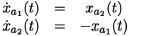
A uniform hysteretic quantization function relates a continuous input trajectory x_i(t) with a piecewise constant output trajectory q_i(t) that satisfies

(4)

and q_i(t₀)= x(t₀). Thus, q_i(t) only changes when it = differs from x_i(t) in ±ΔQ_i. The magnitude ΔQ_i is called quantum. Then, given a time invariant ODE

(5)

where x_a(t) ∈ is the state vector and u(t) ∈ is an input vector, which is a known piecewise constant function, the QSS method (Kofman and Junco, 2001) simulates an approximate system, which is called quantized state system (QSS):

(6)

Here, q(t) is a vector of quantized variables which are quantized versions of the state variables.

Each quantized variable q_i(t) is related with the corresponding state variable x_i(t) with a hysteretic quantization function. Notice that instead of the time step size, we have to choose the quantum ΔQ_i for each state variable.

Since q(t) and u(t) are piecewise constant, the left hand side of (6) (the state derivative ) is also piecewise constant and then the state x(t) is a piecewise linear function of the time. These features allow solving Eq.(6) in a straightforward way, as we did in the introductory example.

A systematic way of simulating Eq.(6) consists ins finding a DEVS model that mimics the behavior of the quantized system. PowerDEVS (Pagliero et al., 2003), is a DEVS simulation software with libraries that implement the complete family of QSS methods.

C. QSS2 and QSS3 Methods

The second order QBI method uses first order quantization. As it is shown in Figure 2, a first order quantizer produces a piecewise linear output trajectory. Each section of that trajectory starts with the value and slope of the input and finishes when it differs from the input in ΔQ_i. A formal definition of a first order quantization funcion can be fouan in (Kofman, 2002).

Figure 2: Trajectories of a first-order quantizer.

The QSS2 method then approximates a system like (5) by (6) but now, the quantized variables q_i(t) follow piecewise linear trajectories and the state variables x_i(t) are piecewise parabolic functions of the time.

The QSS3 method extends the idea of the QSS2 method using second order quantization functions, so that the quantized variable trajectories q_i(t) are piecewise parabolic and the state trajectories x_i are piecewise cubic.

The advantage of QSS2 and QSS3 is that they permit using a small quantum -i.e., a small error tolerance-without increasing considerably the number of calculations. In QSS, the number of steps is inversely proportional with the quantum. In QSS2 it is inversely proportional with the square root of the quantum, and, in QSS3 the number of steps grows with the inverse of the cubic root of the quantum.

D. BQSS and CQSS Method

The BQSS method is similar to QSS, but q_i is always chosen so that x_i(t) goes to q_i(t). It also uses a uniform quantum and the quantized variable qi is restricted so that it never differs from q_i in more than ΔQ_i. The advantage of BQSS is that it permits simulating stiff systems.

CQSS is a blend between BQSS and QSS, that takes the value of q_i equal to the mean of both methods. The method -being appropriate for stiff systems- is also F-stable, i.e., it conserves the stability properties even on the imaginary axis. This feature makes it suitable for the simulation of marginally stable systems (i.e., systems without or with very small damping).

E. Theoretical Properties of QBI Methods

The most important property of the QBI methods is the existence of a global error bound. Given a LTI system where A is a Hurwitz matrix with Jordan canonical form Λ = V⁻¹AV, the error in the QSS methods is always bounded by

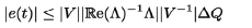(7)

where ΔQ is the vector of quantum adopted at each component (in the case of BQSS and CQSS there is an additional term of error).

Inequality (7) holds for all t, for any input trajectory and for any initial condition. Having a global error bound that can be computed makes a difference between QBI and classic discrete time methods.

III. RELATIVE ERROR CONTROL

In this section, we shall show that using logarithmic quantization, i.e., making the quantum proportional to the magnitude of the quantized variable, QSS methods achieve an intrinsic relative error control.

In order to prove this property, we need first to study the effects of delayed-affine perturbations in a generic LTI system.

A. Ultimate Bound with Affine Perturbations

The following theorem, proven in (Kofman et al., 2007), is an auxiliary result for the main result of this section.

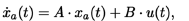
Theorem 1. Consider the system

(8)

where e(t) ∈ , w(t) ∈ , H ∈ and A ∈ is a Hurwitz matrix with Jordan canonical form Λ = V⁻¹AV. Suppose that |w(t)| ≤ w_m for all 0 ≤ t ≤ τ and define

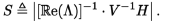(9)

Then, if |V⁻¹e(0)|≤ Swm, then for all 0 ≤ t ≤ τ,

a) |V⁻¹e(t)|≤ S_wm.

b) |e(t)| ≤ |V|S_wm.

The next theorem estimates an ultimate bound for a LTI system with perturbations bounded by an affine delayed function of the state. Particularly, it shows the invariance property of the ultimate bound set estimated by Theorem 3.1 of (Kofman et al., 2008).

Theorem 2. Consider the perturbed system

(10)

where e(t) ∈ , A ∈ is a Hurwitz matrix with Jordan canonical form Λ = V⁻¹AV, H ∈ and the perturbation variable w(t) ∈ satisfies the componentwise bound

(11)

with F ∈ , ∈ , and

(12)

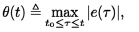
where the maximum is taken componentwise. Define

(13)

suppose that¹ ρ(RF) < 1, and let

(14)

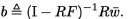
Assume also that θ(t) = 0, ∀t < t₀ and e(t₀) = 0, then, it results that |e(t)| ≤ b, ∀t ≥ t₀.

Proof. Take an arbitrary constant ε > 0.

Suppose for a contradiction that |e(t)| b(1 + ε) for some instant of time t with t₀ < t < ∞ and define t_c as the first instant of time in which this situation occurs:

(15)

Then, we have |e(t)| ≤ b(1 + ε) for t ∈ [t₀,t_c). From Eq.(12) it results that θ(t) ≤ b(1 + ε) for t ∈ [t₀,t_c) and then, using Eq.(11), we obtain

(16)

Taking into account that e(0) = 0 we can apply Theorem 1 with v_m = Fb(1 + ε) + , which results in

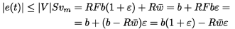
Using the fact that > 0, we finally get

(17)

for t₀ ≤ t <t_c. The continuity of e(t) then contradicts the assumption |e(t)| ≤ b(1 + ε) at time t_c and concludes the proof.

B. Error Bound with Logarithmic Quantization

The basic idea of logarithmic quantization is to take the value of the quantum ΔQ_i proportional to x_i. Since x_i changes continuously with the time, and we do not want the quantum to change continuously, it makes sense to take ΔQ_i proportional to the value of x_i when it last reached an event condition.

Yet, if the quantum is chosen in that way, a problem will occur when x_i evolves near zero. In that case, ΔQ_i will result too small and an unnecessarily large number of events would be produced. Thus, the correct choice for the quantum must have the form:

(18)

where t_k is the last event time in x_i (i.e., t_k ≤ t < t_k+1). As we shall see, E_rel is related to the allowed relative error and ΔQ_min is the minimum quantum.

Then, if we want to simulate a LTI system

(19)

defining 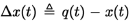, the QSS methods will approximate it by

(20)

Substracting (19) from (20), we obtain the equation for the error e(t) = x(t) − x_a(t):

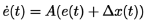(21)

where |Δx(t)| ≤ ΔQ(t) for all t ≥ t₀. Then, taking one component of Δx_i we have

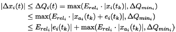
for t_k ≤ t <t_k+1. Taking into account that

and also

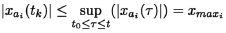
we can apply Theorem 2 to system (21).

Taking H = A, , , and assuming that ρ(RF) < 1, we conclude that

(22)

Calling E_rel to the diagonal matrix with diagonal entries , and ΔQ_min to the vector of minimum quanta, we finally obtain

(23)

It becomes clear that, provided that x_a reaches some large value, the bound on |e(t)| is proportional to that maximum value, i.e., the error bound is relative to the maximum value of x_a. In other words, we have an intrinsic relative error control.

The stability of the numerical solution is ensured by the condition ρ(R · E_rel) < 1, which will be always satisfied for small values of E_rel.

An interesting case occurs when = E_rel for i = 1,...,n, i.e., when we apply the same factor to all the state variables. In that case we obtain the same x(t) expression of (23), but now E_rel is a scalar constant.

In most applications, we shall choose a very small value for E_rel. A typical value would be E_rel = 0.01 or even E_rel = 0.001. In that case, we can approximate Eq.(23) as:

(24)

It is worth to remark that we have analyzed a global error property, which is only valid for stable LTI systems. In general, global error properties cannot be ensured for unstable systems as the error grows with the advance of the time. In the case of marginally stable systems, the error in QSS schemes is bounded by a linear growing function of the time (Kofman and Zeigler, 2005).

IV. EXAMPLES

The following examples were implemented and simulated with PowerDEVS using a notebook PC running under Windows XP with a 933MhZ Pentium III processor.

A. Mass-Spring-Damper System

The LTI system

(25)

represents a mass-spring-damper system with an external force u₀(t). In this experiment, we shall consider that

(26)

Taking parameters k = m = b = 1, and selecting E_rel = 0.01, ΔQ_min = 0.001 in both state variables, the simulation with the QSS2 method gives the result shown in Figure 3.

Figure 3: Spring—Mass System Trajectories

Since the system is LTI, we can calculate the maximum error following the analysis of Section B. In this case, Eq.(23) results:

where x_max and v_max are the maximum absolute value reached by x and v in Eq.(25).

Then, it results that the error in each variable is theoretically bounded by

(27)

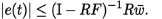
Figure 4 corroborates this bound for x(t). It also compares the absolute error |e_x(t)| with the magnitude that bounds the quantum E_rel|x(t)|, showing that there is a close relationship between these quantities.

Figure 4: Absolute error

If uniform quantization were used, the error in Figure 4 would have been bounded by a constant instead of being bounded by a signal proportional to the actual value of the state.

The number of steps performed by the simulation was 115 and 156 in x and v, respectively. A similar number of steps using QSS2 with uniform quantization can be obtained selecting ΔQ = 0.01. However, the simulation with this quantum provokes an important relative error when the trajectories cross near zero.

Moreover, if we increase the force u₀(t) by a factor of 100, the simulation with logarithmic quantization using the same settings than before performs almost the same number of steps (there are only 50 additional steps, i.e., a 18% increase). The simulation with uniform quantization, however, multiplies by 10 the number of steps (i.e., a 1000% increase).

In other words, the computational costs using logarithmic quantization is almost independent of the magnitude of the signals, while using uniform quantization, the costs are highly dependent on these magnitudes.

B. 80th order marginally stable stiff nonlinear system

The following system of equations represents a lumped model of a lossless LC transmission line where L = C = 1, with a nonlinear load at the end:

(28)

We consider an input pulse entering the line, u₀, given by Eq.(26), and a nonlinear load with a law g(u_n(t)) = (10000 · u_n)³. We also set null initial conditions u_i = φ_i = 0.

We consider 40 LC sections (i.e., n = 40), which results in a 80^th order system. The linearization around the origin (u_i = φ_i = 0), shows that the system is marginally stable (the linearized model does not have any damping term). Also, the system is stiff (the nonlinear load adds a fast mode when u_n grows).

We decided to simulate the system of Eq.(28) using the F-stable CQSS method with logarithmic quantization with E_rel = 0.01 and ΔQ_min= 0.0001 in all the state variables.

To obtain the first 100 seconds of simulated time, CQSS needed about 47 seconds. Figure 5 shows the voltage at the 35^th section of the line (i.e., near the load end).

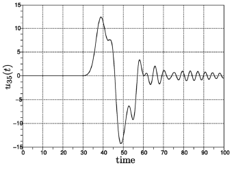
Figure 5: CQSS simulation of System (28)

In order to analyze the accuracy of the results, we simulated the system with Matlab's ode15s method (ode15s was the best Matlab algorithm for this example) using a very small error tolerance (we set the relative and absolute error to 1 × 10⁻¹²). We found that the results obtained with CQSS are very similar to those obtained with ode15s, and they cannot be distinguished with the naked eye.

Increasing the amplitude of the input pulse by a factor of 100, the simulation time grows to 86 seconds. Increasing it again by a factor of 100 (i.e., selecting u(t) = 100000) the simulation time becomes 125 seconds.

Using uniform quantization, in order to get a similar accuracy, we need to select ΔQ = 0.01 in all the state variables except for the one corresponding to u₃₉, where the signal is too small and an appropriate value is ΔQ = 0.0001. Although with this choice we get faster results (about 18 seconds), whenever we increase the input amplitude by a factor of 100, the simulation time also increases about this factor.

This analysis shows that logarithmic quantization can be used with any QBI method and it works providing a selected accuracy irrespective of the signal amplitudes (which are usually unknown before the simulation is performed).

On the other hand, uniform quantization depends strongly on the system and its input signals and initial conditions. In many cases, if we do not know anything about the system trajectories, it is almost impossible to select an appropriate uniform quantum.

V. CONCLUSIONS

We introduced a modification to QSS methods, where the quantum grows and decreases proportional to the magnitude of the corresponding state variable. We showed that this strategy produces an intrinsic relative error control, in contrast to the absolute error control associated to the use of uniform quantization.

The main advantage of the proposed methodology is that a user can select directly the relative tolerance of a simulation without a prior knowledge about the system trajectories. This idea makes QSS methods more robust and much easier to use, without sacrifying accuracy or computational efficience.

VI. ACKNOWLEDGE
This work was partially supported by ANPCYT grant PICT2005 -31653.

---

¹ We call ρ(RF) to the spectral radius of matrix RF, i.e., the maximum absolute value of its eigenvalues. The condition ρ(RF) < 1 means that the eigenvalues of RF are inside the unit circle and it ensures that (I − RF) is invertible

REFERENCES
1. Cellier, F. and E. Kofman, Continuous System Simulation, Springer, New York (2006).         [ Links ]
2. Elmqvist, H., D. Brueck, and M. Otter. Dymola User's Manual. Dynasim AB, Research Park Ideon, Lund, Sweden (1995).         [ Links ]
3. Hairer, E., S. Norsett, and G. Wanner, Solving Ordinary Differential Equations I. Nonstiff Problems, Springer, 2nd edition (1993).         [ Links ]
4. Hairer, E. and G. Wanner, Solving Ordinary Differential Equations II. Stiff and Differential-Algebraic Problems, Springer, 1st edition (1991).         [ Links ]
5. Kofman, E., "A Second Order Approximation for DEVS Simulation of Continuous Systems," Simulation, 78, 76-89 (2002).         [ Links ]
6. Kofman, E., "Discrete Event Simulation of Hybrid Systems," SIAM Journal on Scientific Computing, 25, 1771-1797 (2004).         [ Links ]
7. Kofman, E., "A Third Order Discrete Event Simulation Method for Continuous System Simulation," Latin American Applied Research, 36, 101-108 (2006).         [ Links ]
8. Kofman, E., H. Haimovich, and M. Seron, "A systematic method to obtain ultimate bounds for perturbed systems," International Journal of Control, 80, 167-178 (2007).         [ Links ]
9. Kofman, E. and S. Junco, "Quantized State Systems. A DEVS Approach for Continuous System Simulation," Transactions of SCS, 18, 123-132 (2001).         [ Links ]
10. Kofman, E., M. Seron, and H. Haimovich, "Control Design with Guaranteed Ultimate Bound for Perturbed Systems," Automatica, 44, 1815-1821 (2008).         [ Links ]
11. Kofman, E. and B. Zeigler, "DEVS Simulation of Marginally Stable Systems,"Proceedings of IMACS'05, Paris, France (2005).         [ Links ]
12. Migoni, G., E. Kofman, and F. Cellier, "Integración por Cuantificación de Sistemas Stiff," Revista Iberoam. de Autom. e Inf. Industrial, 4, 97-106 (2007).         [ Links ]
13. Pagliero, E., M. Lapadula, and E. Kofman, "PowerDEVS. Una Herramienta Integrada de Simulación por Eventos Discretos," Proceedings of RPIC'03,, San Nicolas, Argentina 1, 316-321 (2003).         [ Links ]
14. Shampine, L. and M. Reichelt, "The MATLAB ODE Suite," SIAM Journal on Scientific Computing, 18, 1-22 (1997).         [ Links ]
15. Zeigler, B., T. Kim, and H. Praehofer, Theory of Modeling and Simulation. Second edition, Academic Press, New York (2000).         [ Links ]

Received: October 18, 2007.
Accepted: July 2, 2008.
Recommended by Guest Editors D. Alonso, J. Figueroa, E. Paolini and J. Solsona.