Estimation of the particle size distribution of a dilute latex from combined elastic and dynamic light scattering measurements. A method based on neural networks

G.S. Stegmayer^†, V.D. Gonzalez^‡, L.M. Gugliotta^‡, O.A. Chiotti^† and J.R. Vega^†,‡

^† CIDISI (UTN - Facultad Regional Santa Fe), Santa Fe, Argentina,
gstegmayer@santafe-conicet.gov.ar, chiotti@ santafe-conicet.gov.ar, jvega@ santafe-conicet.gov.ar
^‡ INTEC (UNL - CONICET), Santa Fe, Argentina,
veronikg@ santafe-conicet.gov.ar, lgug@intec.unl.edu.ar

Abstract — A method for estimating the particle size distribution (PSD) of a dilute latex from light scattering measurements is presented. The method utilizes a general regression neural network (GRNN), that estimates the PSD from 2 independent sets of measurements carried out at several angles: (i) light intensity measurements, by elastic light scattering (ELS); and (ii) average diameters measurements, by dynamic light scattering. The GRNN was trained with measurements simulated on the basis of typical asymmetric PSDs (unimodal normal-logarithmic distributions of variable mean diameters and variances). First, the ability of the method was tested on the basis of two synthetic examples. Then, the obtained GRNN was used for estimating the PSD of a narrow polystyrene (PS) latex standard of nominal diameter 111 nm. The standard was also characterized by 2 independent techniques: capillary hydrodynamic fractionation, and transmission electron microscopy (TEM). The PSD predicted by the GRNN resulted close to that obtained by TEM. The estimated PSDs were better than those obtained through standard numerical techniques for 'ill-conditioned' inverse problems.

Keywords — Elastic Light Scattering. Dynamic Light Scattering. Particle Size Distribution. Neural Network. Inverse Problems

I. INTRODUCTION

The particle size distribution (PSD) of a polymer latex is an important morphological characteristic that determines the processability and end-use properties of the material when used as an adhesive, a coating, an ink, or a paint. Transmission electron microscopy (TEM) is the main reference technique for directly observing and measuring the PSD. However, it is experimentally expensive, time-consuming, and difficult, mainly when analyzing soft latexes and/or broad PSDs. Also, the electron beam can produce a sample damage or a size contraction; and the PSD evaluation may involve counting thousands of particles (Llosent et al., 1996).

Several fractionation techniques (such as capillary hydrodynamic fractionation -CHDF-, field flow fractionation, hydrodynamic chromatography, and disc centrifugation), are also employed for measuring the PSDs. In particular, CHDF separates the particles according to their size, and employs a turbidity detector for determining the number of particles of each eluted fraction. CHDF is an indirect technique, since it requires a particle diameter calibration usually based on the analysis of narrow standards. Even though it is presented as a high resolution technique, it normally produces broad PSDs, as a consequence of the instrumental broadening that mainly occurs in the capillary tube (Silebi and Dos Ramos, 1989).

The so-called ensemble techniques are based on simultaneously measuring all particles in their media without previous fractionation. They include, acoustic-attenuation spectroscopy and focused-beam reflectance measurements, for concentrated systems (e.g., Scheffold et al., 2004; Li and Wilkinson, 2005); and several optical techniques such as turbidimetry, elastic light scattering (ELS), and dynamic light scattering (DLS) (Pecora, 1985; Llosent et al., 1996; Vega et al., 2003a,b). Particles in the sub-micrometer range are frequently measured by ELS and DLS (Bohren and Huffman, 1983; Chu, 1991). The instruments are similar, and basically consist of a monochromatic laser light falling onto a dilute latex sample. A photometer placed at a given detection angle, θ_r, with respect to the incident light, collects the light scattered by the particles over a small solid angle. In ELS, the light intensity, I(θ_r), is measured at each θ_r (r=1,2,...,R). The ELS measurement model is given by:

(1)

where f(D) is the (unknown) PSD (represented as number of particles vs. diameter (D); and C_I(θ_r, D) is the light intensity scattered by a particle of diameter D at θ_r, and it is calculated through the Mie scattering theory (Bohren and Huffman, 1983; Glatter et al., 1985).

In DLS, a devoted digital correlator measures (at each θ_r) the second-order autocorrelation functions of the scattered light, , for different values of the time delay, ξ.. This measurement is related to the (first-order and normalized) autocorrelation function of the electric field, , through:

(2.a)

where is the measured baseline; and β (<1) is an instrumental parameter. Then, the DLS measurement model is given by (see e.g., Vega et al., 2003b):

(2.b)

with

(2.c)

where λ (nm) is the in-vacuo wavelength of the incident laser light; n_m is the refractive index of the non-absorbing medium; k (=0.0138gnm²/s²K) is the Boltzmann constant; T (K) is the absolute temperature; and η (g /nm s) is the medium viscosity at the given T.

The two measurement models of Eqs. (1) and (2) are represented by Fredholm equations of the first kind; and the estimation problem consists in finding f(D) through the inversion of: a) Eq. (1) from the knowledge of I(θ_r), in the ELS problem; and b) Eq. (2.b) from the knowledge of , in the DLS problem. Such inverse problems are typical of most measurement systems where only indirect measurements are available. Inverse problems are normally 'ill-conditioned'; i.e., small errors in the measurement (for example, small perturbations due to the measurement noise), can originate large changes in the f(D) estimate. Regularization methods aim at improving the numerical inversion by including adjustable parameters, a priori knowledge of the solution, or some smoothness conditions (Engl et al., 1996; Tikhonov and Arsenin, 1977). While a strong regularization will produce an excessively smoothened and wide PSD, a weak regularization will originate oscillatory PSD estimates. Then, a trade-off solution must be selected.

Unfortunately, all light scattering measurements are recognized to have low information content on the PSD; and consequently only a rather poor resolution is expected. Combination of two or more independent sets of measurements allows increasing the information content, and can contribute to improving the quality of the PSD estimate (Eliçabe and Frontini, 1996; Frontini and Eliçabe, 2000; Vega et al., 2003a).

Several neural network (NN) methods have also been applied for solving inverse problems in light scattering systems. For instance, radial basis function (RBF) NNs proved adequate for simultaneously estimating the average radius and the particle refractive index in a system with homogeneous spheres (Ulanowski et al., 1998). Multilevel NNs with linear activation functions have been used for simultaneously estimating the size and parameters representative of the PSD shape, in binary mixtures of particles (e.g., spheroids and cylinders). However, as far as the authors are aware, no NN-based method has yet been published for estimating the complete PSD.

In this work, a novel method that combines ELS and DLS measurements is proposed to estimate the PSD of a latex. The estimation model is implemented through a NN, that is trained with a large set of typical asymmetric PSDs and their corresponding simulated measurements. The method is then evaluated through both synthetic and experimental examples.

II. THE PROPOSED METHOD

In principle, Eqs. (1, 2) can be combined in a single inversion problem for estimating the PSD from both sets of measurements. To this effect, a scalar value [I(θ_r)] must be combined with a complete function [], at each θ_r. Since each individual inversion problem (ELS and DLS) is 'ill-conditioned', their combination in a single inversion problem will be ill-conditioned too. As an alternative, we suggest to replace Eqs. (2.b,c) by the expression corresponding to the average diameter typically calculated in a DLS measurement at each θ_r, D_DLS(θ_r). These diameters can be calculated on the basis of  computed from Eq. (2.a), through the cumulants method by Koppel (1972). At each θ_r, D_DLS(θ_r) is usually reported by the standard software included in the commercial equipments.

For a given PSD, D_DLS(θ_r) can be theoretically calculated through the following expression:

(3)

For a monodisperse PSD (i.e., all particles of the same diameter, D₀), then D_DLS(θ_r) = D₀, for all θ_r. In contrast, for a wide PSD with distributed diameters, D_DLS(θ_r) varies with θ_r according to Eq. (3).

Assume now that the D-axis is discretized in N points {D₁, ..., D_N} at regular intervals ΔD, in a given diameter range [D_min-D_max]. Similarly, the detection angle θ is discretized in R points {θ₁, ..., θ_R} at regular intervals Δθ, in the diameter range [θ_min-θ_max]. In the defined grids for θ and D, Eqs. (1) and (3) can be rewritten as:

(4.a)

(4.b)

Then, the estimation problem consists in finding the PSD ordinates f(D_i) [in Eqs. (4)], from the knowledge of both indirect measurements: I(θ_r) and D_DLS(θ_r). In this work, such inverse problem will be solved through a NN-based model.

A. The NN Inverse Model

Consider an arbitrary system with 'n' input variables and 'm' output variables; and call x (= [x₁, ..., x_n]^T) and y (= [y₁, ..., y_m]^T) the input and output vectors, respectively. A NN model is useful for describing the input/output performance of such a system, from the knowledge of several {x, y} pairs.

A RBF NN has a simple architecture with only one hidden layer (Cybenko, 1996). The activation function of the j-th hidden unit depends on the Euclidean distance (d) between the input vector x and a reference vector c_j, defined as the center of the neuron. The most common shape of such activation functions is a Gaussian that exhibits a radial symmetry around c_j. Then, the NN model that relates the output of the j-th hidden neuron, h_j, with the input vector x is evaluated through the following expression:

(5)

The k-th output of a RBF network, y_k, is simply a weighted linear combination of the basis functions, i.e.:

(6)

A general regression neural network (GRNN) is a particular case of a RBF network. The GRNN is a normalized RBF network in which there is a hidden unit centered at every training case (Specht, 1991); thus the number of neurons equals the number of input/target vectors in the training set. The GRNN is a one-pass learning algorithm with a highly parallel structure. Even with sparse data in a multidimensional measurement space, the algorithm provides smooth transitions from one observed value to another (Specht, 1991).

The hidden-to-output weights (w_kj) are just the target values, so the output is simply a weighted average of the target values of training cases close to the given input case. The parameters to be learned are the widths of the units RBF (also called "smoothing parameters" or "spreads"), and often a single width is used. When the spread is defined as 1.177 times the Gaussian standard deviation (σ_G), then: 1) if d = 0 (i.e., c_j ≡ x), then h_j = 1; and 2) if d=σ_G, then h_j = 0.5.

Let us assume that we have trained the GRNN model with a training set containing the input/target pairs {x_i, t_i}. Also, assume that the network receives an input value x which is close to x_i. Then, the corresponding hidden layer output will be close to 1; and the output layer response will be close to t_i.

If a large spread is adopted, then the area around the input vector where hidden layer neurons will respond with significant outputs will be larger. On the contrary, if the spread is small, the RBF is narrow, and the neuron with the centroid closest to the input will have the largest output. Thus, the network will tend to respond with the target vector associated with the nearest design input vector. As spread becomes larger, the RBF is wider and several neurons will respond to an input vector. In summary, the network will produce a weighted average between target vectors whose design input vectors are closest to the new input vector. As spread becomes larger, more neurons will contribute to the average, and therefore the network function becomes smoother (Wasserman, 1993).

Before training the network, the centers of the hidden neurons must be chosen. To maximize accuracy, each training input is made to be a center, and therefore the number of hidden nodes in the GRNN model coincides with the number of training vectors.

B. The GRNN Training Stage

The NN was trained on the basis of a set of discrete PSDs, and their corresponding measurements obtained from Eqs. (4). To simplify the problem, the D and θ discrete axes will be assumed as fix; and therefore only the ordinates of f(D_i), D_DLS(θ_r), and I(θ_r) will be processed by the network. Each a priori known f(D_i) was placed in the diameter range [50-1100] nm, at regular interval ΔD = 5 nm. In all cases, the measurements were taken in the θ-range [20°-140°], at regular intervals of Δθ = 10°. Thus, the input vector is obtained by stacking I(θ_r) and D_DLS(θ_r), each represented by R = 13 discrete points, and the total number of input points to the model is 2'R = 26. The output variables, f(D_i), resulted of N = 211 points.

Ideally, training data must be generated with the criterion of covering all possible PSDs. In our case, we have restricted the PSDs to only follow a log-normal distribution, given by:

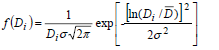(7)

where D_i (i=1, 2, ..., 211) represents each discrete diameter;  is the geometric mean diameter; and σ is the standard deviation.

For generating the training set,  was varied in the range [80-1000] nm, each 5 nm. At each , 20 distributions were generated, with standard deviations in the range [0.01-0.20] nm, each 0.01 nm. Hence, 185 different  values were considered, with 20 PSDs at each point, yielding a total of 3700 training patterns. All patterns were normalized to fall in the range [0,1]. The network perfectly learned the training data, with an approximate root mean square error (RMSE) of 10^-7.

III. NN-MODEL VALIDATION

Two kind of validations were implemented. First, the GRNN was validated through simulated or "synthetic" examples, since in these cases the solutions are "a priori" known, and therefore the NN performance can be clearly evaluated. Then, the model was tested through an experimental example that involved a polystyrene (PS) latex of narrow PSD and known nominal diameter. In this case, the "true" PSD is unknown; but the best approximation is given by an independent PSD measurement as obtained from TEM.

A. Validation with simulated examples

Two asymmetric and unimodal PSDs of a PS latex were simulated. The first PSD, f₁(D), follows a log-normal distribution as given by Eq. (7), with  = 205 nm, and σ₁ = 0.115 nm. The second PSD was assumed to follow an exponentially-modified Gaussian (EMG) distribution, that is obtained by convoluting a (symmetric) Gaussian distribution (of mean diameter  and standard deviation σ₂), with a decreasing exponential function (of decay constant, τ), i.e.:

(8)

where the symbol '*' represents the "convolution product". In this example, the following parameters were adopted:  = 340 nm; σ₂ = 20 nm; and τ = 10 nm.

Both selected PSDs are represented in Fig 1.a). The log-normal PSD belongs to the class of distributions used for training the NN, and therefore it will be useful for evaluating the model interpolation ability. In contrast, the EMG PSD can exhibit a high asymmetry, and was selected to evaluate the ability of the network for estimating a PSD that differs in shape from those used during the training stage.

Figure 1. a) "True" (thick trace) and estimated (thin trace) PSDs; b) scattered intensity measurements (by ELS); and c) average diameters (by DLS).

To simulate the ELS and DLS measurements, we assumed that the light scattering photometer is fitted with a vertically-polarized He-Ne laser. At the laser wavelength (632.8 nm), the particle refractive index is n_p = 1.5729, and the medium (pure water) refractive index is n_m = 1.3319. From these parameters, the C_I(θ_r,D_i) coefficients can be evaluated through the Mie theory (Bohren and Huffman, 1983). The noise-free measurements were simulated through Eqs. (4). Then, random Gaussian noises were added to each measurement. The noise standard deviations were selected as those typically found in measurements taken from a commercial equipment, i.e.: i) 1.0% of the signal maximum, for I(θ_r); and ii) 0.32% of the signal maximum, for D_DLS(θ_r).

In Fig. 1.a), the PSDs f₁(D) and f₂(D), are represented by a continuous thick line. In Figs. 1.b,c), the noise-free measurements (in continuous line), and the noisy measurements (in symbols), are shown. From the noisy measurements, the trained GRNN predicted the PSDs, and , represented (in thin trace) in Fig. 1.a). As expected, the prediction of f₁(D) resulted much better than the prediction of f₂(D).

B. Experimental validation

A commercial latex standard of PS and nominal diameter 111 nm was measured through the following techniques: 1) DLS; 2) ELS; 3) CHDF; and 4) TEM. The PSDs obtained from TEM and CHDF were previously reported by Gugliotta et al. (2000); and are reproduced in Fig. 2a).

Figure 2. a) Estimated PSDs; b) average diameters (by DLS): measurements (in symbols); simulations from the estimated PSDs (in continuous traces).

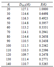
The DLS measurements were implemented with a laser light-scattering photometer (Brookhaven Instruments, Inc.), fitted with a vertically polarized He-Ne laser (at 632.8 nm), together with a digital correlator (model BI-2000 AT). The PS latex was diluted to avoid multiple scattering, and the measuring times ranged between 200 and 500 s. The measurements were carried out at 30 C; and at the following detection angle range: [20°-140°], evenly-spaced each Δθ = 10°.

From Eq. (2), was calculated, and the average diameters D_DLS(θ_r) (see Table 1) were obtained through the second-order cumulants method (Koppel, 1972). The I(θ_r) measurements (see Table 1) were indirectly derived from the baselines, through: , where I(20) = 1 was adopted as the reference intensity. The measurements of Table 1 were fed into the trained GRNN; and the resulting estimated PSD is indicated as "NN" in Fig. 2a).

Table 1. DLS and ELS measurements.

Alternatively, the PSD can be directly estimated from the ELS measurements, I(θ_r), by numerically inverting Eq. (4.a). To this effect, Eq. (4.a) was first converted into the following vector expression:

(9)

where i = [I(θ₁), ..., I(θ_R)]^T is a (R×1) vector containing the ordinates of I(θ), at the R selected discrete angles; f = [f(D₁), ..., f(D_N)]^T is a (N×1) vector containing the ordinates of f(D) at the N discrete diameters; and C_I is a (R×N) matrix containing the corresponding Mie coefficients.

To solve Eq. (4.a), the Phillips-Tikhonov regularization technique was applied (Tikhonov and Arsenin, 1977). Since C_I is an ill-conditioned matrix, then a regularized pseudo-inverse of C_I may be computed through: C_I^[-1] = (C_I^T C_I + α H)^-1 C_I^T, where H is a regularization matrix (Tikhonov and Arsenin, 1977), and α is an adjustable parameter. Thus, the vector form of the estimated PSD, , can be obtained by inverting Eq. (9) as follows:

(10)

The inversion method of Eq. (10) was applied onto the measured I(θ_r) of Table 1; and the regularization parameter α was adjusted by trial-and-error, in order to obtain the better possible solutions (i.e., the lower α value that produces positive estimates of the PSD ordinates). The estimated PSD is indicated as "ELS" in Fig. 2a).

A visual comparison of the four PSDs indicates that the NN solution is a good approximation to the "better" estimation obtained by TEM. In contrast, CHDF and ELS estimates are clearly wider than TEM; and additionally, the ELS estimate exhibits a secondary population (of a high mean diameter) not revealed by TEM. Note that the numerical inversion of Eq. (10) only included information on the ELS measurement; and in such sense the information content is lower than in the case of the GRNN method.

From the PSDs of Fig. 2a), the corresponding average diameters D_DLS(θ_r) were calculated through Eq. (4.b); and are represented in Fig. 2b). Additionally to D_DLS(90°), Table 2 summarizes some characteristic mean diameters of a PSD, such as the standard number-mean diameter, D_1,0, and the D_6,5 diameter, defined by:

;

(11)

Table 2. Comparison of average diameters.

The D_6,5 diameter approaches D_DLS(90°) for particles in the Rayleigh scattering regime, typically observed for particles with D < 100 nm. For this reason, D_6,5D_DLS(90°) for the PSDs obtained by NN and TEM (see Table 2).

The prediction of D_DLS(θ_r) from the PSD estimated by the NN is close to the experimental points determined by DLS (symbols in Fig. 2b). This result also supports the idea of the quality of the estimation of the PSD through the method here proposed.

IV. CONCLUSIONS

A NN for estimating the PSD of a PS latex from combined ELS and DLS measurements was developed. The proposed model uses a GRNN that was trained on the basis of simulated log-normal PSDs, with particles in the diameter range [50-1100] nm.

The method was successfully evaluated on the basis of both synthetic and experimental examples. It was observed that the trained network was able of: a) adequately recuperating the log-normal and EMG PSDs; and b) estimating narrow PSDs of commercial PS standards, with improved results with respect to CHDF measurements. The NN also provided better results than those obtained by solving the inverse problem related to the ELS measurements.

The trained GRNN is a fast and robust tool. With respect to the standard inversion techniques, the network presents the advantages of not requiring any numerical inversion or parameter adjustment; and it is relatively insensitive to standard noisy measurements. The success of the model is mainly due to the increased information content gained through the measurement combination. Although not shown, the performance of a GRNN developed only on the basis of ELS measurements was rather poor.

The main limitation of the model is the imposed restriction to unimodal PSDs in the selected diameter range. However, the network performance can be significantly improved by increasing the number of simulated experiments used during the training stage. For example, the accuracy of the PSD estimate could be improved by including a large spectrum of PSD shapes (e.g., bimodals PSDs), or by increasing the PSD resolution by training the network with lower discretization intervals (either ΔD or Δθ).

ACKNOWLEDGEMENTS
To CONICET, MinCyT, Universidad Tecnológica Nacional (Facultad Regional Santa Fe), and Universidad Nacional del Litoral, for the financial support.

REFERENCES
1. Bohren, C.F. and D.R. Huffman, Absorption and Scattering of Light by Small Particles, John Willey & Sons, New York (1983).         [ Links ]
2. Chu, B., Laser Light Scattering, Academic Press, New York (1991).         [ Links ]
3. Cybenko, G. "Neural networks in computational science and engineering", IEEE Comp. Sci. and Eng., 3, 36-42 (1996).         [ Links ]
4. Eliçabe, G.E. and G.L. Frontini, "Determination of the particle size distribution of latex using a combination of elastic light scattering and turbidimetry: A simulation study", J. Coll. Interf. Sci., 181, 669-672 (1996).         [ Links ]
5. Engl, H.W., M. Hanke and A. Neubauer, Regularization of Inverse Problems, Kluwer Academic Publishers, Dordrecht, The Netherlands (1996).         [ Links ]
6. Frontini, G.L. and G.E. Eliçabe, "Combination of indirect measurements to improve signal estimation", Lat. Amer. Appl. Res., 30, 99-105 (2000).         [ Links ]
7. Glatter, O., M. Hofer, C. Jorde and W. Eigner, "Interpretation of elastic light-scattering data in real space", J. Coll. and Interf. Sci., 105, 577-586 (1985).         [ Links ]
8. Gugliotta, L.M., J.R. Vega, J.R. Leiza and G.R. Meira, "Distribuciones de tamaños de partícula por fraccionamiento hidrodinámico capilar. Calibración del ensanchamiento instrumental", Proc. del VII Simposio Latinoamericano de Polímeros (SLAP 2000), La Habana, Cuba, 408 (2000).         [ Links ]
9. Koppel, D.E. "Analysis of macromolecular polydispersity in intensity correlation spectroscopy: the method of cumulants", J. Chem. Phys., 57, 4814-4820 (1972).         [ Links ]
10. Llosent, M.A., L.M. Gugliotta, and G.R. Meira, "Particle size distribution of SBR and NBR latexes by UV-vis turbidimetry near the Rayleigh region", Rubber Chem. and Tech., 69, 696-712 (1996).         [ Links ]
11. Li, M. and D. Wilkinson, "Determination of non-spherical particle size distribution from chord length measurements. Part 1: Theoretical analysis", Chem. Eng. Sci., 60, 3251-3265 (2005).         [ Links ]
12. Pecora, R., Dynamic Light Scattering. Applications of Photon Correlation Spectroscopy, Plenum Press, New York (1985).         [ Links ]
13. Scheffold, F., A. Shalkevich, R. Vavrin, J. Crassous and P. Schurtenberger, "PCS particle sizing in turbid suspensions: scope and limitations"; in Particle Sizing and Characterization, T. Provder and J. Texter, Ed.; ACS Symp. Series, 881, 3-32 (2004).         [ Links ]
14. Silebi, C. A. and J. G. Dos Ramos, "Axial dispersion of submicron particles in capillary hydrodynamic fractionation" AIChE J., 35, 1351-1364 (1989).         [ Links ]
15. Specht, D.F. "A generalized regression neural network", IEEE Trans. Neural Networks, 2, 568-576 (1991).         [ Links ]
16. Tikhonov, A.N. and V. Arsenin, Solution of Ill-posed Problems, Wiley, New York (1977).         [ Links ]
17. Ulanowski, Z., Z. Wang, P. Kaye and I. Ludlow, "Application of neural networks to the inverse light scattering problem for spheres", Appl. Optics, 37, 4027-4033 (1998).         [ Links ]
18. Vega, J.R., G.L. Frontini, L.M. Gugliotta and G.E. Eliçabe, "Particle size distribution by combined elastic light scattering and turbidity measurements. A novel method to estimate the required normalization factor", Part. & Part. System Charact., 20, 361-369 (2003a).         [ Links ]
19. Vega, J.R., L.M. Gugliotta, V.D.G. Gonzalez and G.R. Meira, "Latex particle size distribution by dynamic light scattering. A novel data processing for multi-angle measurements", J. of Col. and Int. Sci., 261, 74-81 (2003b).         [ Links ]
20. Wasserman, P.D. Advanced Methods in Neural Computing, New York: Van Nostrand Reinhold, (1993).         [ Links ]

Received: October 18, 2007.
Accepted: July 20, 2008.
Recommended by Guest Editors D. Alonso, J. Figueroa, E. Paolini and J. Solsona.