ARTICLES

Numerical simulation of the flow around the ahmed vehicle model

G. Franck^1,2, N. Nigro², M. Storti² and J. D'Elía²

¹ Universidad Tecnológica Nacional (UTN), Facultad Regional Santa Fe (FRSF)
Lavaise 610, 3000-Santa Fe, Argentina, gfranck@intec.unl.edu.ar, http://www.utn.edu.ar
² Centro Internacional de Métodos Computacionales en Ingeniería (CIMEC)
Instituto de Desarrollo Tecnológico para la Industria Química (INTEC)
Universidad Nacional del Litoral -CONICET , Güemes 3450, 3000-Santa Fe, ARGENTINA
ph.: (54342)-4511 594/5, fx: (54342)-4511 169
(nnigro, mstorti, jdelia)@intec.unl.edu.ar http://www.cimec.org.ar

Abstract - The unsteady flow around the Ahmed vehicle model is numerically solved for a Reynolds number of 4.25 million based on the model length. A viscous and incompressible fluid flow of Newtonian type governed by the Navier-Stokes equations is assumed. A Large Eddy Simulation (LES) technique is applied together with the Smagorinsky model as Subgrid Scale Modeling (SGM) and a slightly modified van Driest near-wall damping. A monolithic computational code based on the finite element method is used, with linear basis functions for both pressure and velocity fields, stabilized by means of the Streamline Upwind Petrov-Galerkin (SUPG) scheme combined with the Pressure Stabilizing Petrov-Galerkin (PSPG) one. Parallel computing on a Beowulf cluster with a domain decomposition technique for solving the algebraic system is used. The flow analysis is focused on the near-wake region, where the coherent macro structures are estimated through the second invariant of the velocity gradient (or Q-criterion) applied on the time-average flow. It is verified that the topological features of the time-average flow are independent of the averaging time T and grid-size.

Keywords - Ahmed Vehicle; Bluff Aerodynamics; Incompressible Viscous Fluid; Large Eddy Simulation (LES); Time-Average Flow; Finite Element Method; Fluid Mechanics.

I. INTRODUCTION

A. The Ahmed vehicle model

Ground vehicles can be classified as bluff-bodies that move close to the road surface and are fully submerged in the fluid. In general, for the usual velocities of commercial passenger cars, buses and trucks, compressible effects can be neglected and an incompressible viscous fluid model can be assumed. As the Reynolds numbers based on the body length are usually too high, the flow regimes are fully turbulent. In addition, a key feature of the flow field around a ground vehicle is the presence of several separated flow regions, while the net aerodynamic force is the result of complicated interactions among them. Even simple basic vehicle configurations with smooth surfaces, free from appendages and wheels, generate a variety of quasi two dimensional and fully three dimensional regions of separated flows where the largest one is the wake. In a time-averaged sense, the separated flow regions exhibit complicated kinematic macro structures and those present in the wake determine mostly the body drag. Nowadays, numerical simulations, wind tunnel and road tests are jointly used in the automotive industry for the aerodynamic study from several perspectives.

The Ahmed vehicle model is a very simplified bluff-body which is frequently employed as a benchmark in vehicle aerodynamics. It has been used in several experiments (Ahmed et al., 1984; Sims-Williams, 1998; Bayraktar et al., 2001; Spohn and Gilliéron, 2002; Lienhart and Becker, 2003) and numerical studies (Han, 1989; Basara et al., 2001; Basara, 1999; Basara and Alajbegovic, 1998; Gilliéron and Chometon, 1999; Kapadia et al., 2003). A slightly modified version was also studied by Duell and George (1999); Barlow et al. (1999); Krajnović and Davidson (2003).

The shape of this body is free from all accessories and wheels but it still retains the primary behavior of the vehicle aerodynamics, as seen in Fig. 1. Special attention is focused on the time-averaged flow in the near-wake and the dependence of drag on the slant angle α at the top rear end. The rear end is a simplification of a so-called fastback one such as on a Volkswagen Golf I. This model was tested in open jet wind tunnels and no velocity distributions were reported in the inlet and outlet boundaries (Ahmed et al., 1984). Previous numerical simulations had assumed the incoming flow to be laminar and steady (Han, 1989; Krajnović and Davidson, 2004; Basara and Alajbegovic, 1998). Wind tunnel experiments on this model show two critical slant angles: α_m≈12.5° and α_M≈30.0°, called first and second critical angles, respectively, where the main topological structure of the time-averaged flow in the near-wake changes significantly as summarized in Table 1 (Ahmed et al., 1984; Sims-Williams, 1998; Bayraktar et al., 2001; Spohn and Gilliéron, 2002; Lienhart and Becker, 2003).

Figure 1: Ahmed model, dimensions in mm.

Table 1: Time-averaged flow in the near-wake of the Ahmed vehicle as a function of the slant angle α, where α_m≈12.5° and α_M ≈ 30.0°.

Among the experimental tests, Janssen and Hucho (1975) showed the dependence of the flow on the slant angle at the rear end for an industrial vehicle model, while Morel (1978) performed tests on the Morel body which is previous to the Ahmed one. Both models represent two benchmarks widely used in the automotive industry (Basara and Alajbegovic, 1998).

On one hand, among numerical simulations, a LES around a bus-like vehicle is developed by Krajnović (2002), Krajnović and Davidson (2003), while Gilliéron and Spohn (2002) showed a Detached Eddy Simulations (DES) over another simplified vehicle model. Other sources of related work can be found in Hucho (1998) and ERCOFTAC (2007).

Regarding numerical benchmarks with the present model, several computations were performed using the Reynolds Averaged Navier-Stokes (RANS) equations (Han, 1989; Basara et al., 2001; Basara, 1999; Basara and Alajbegovic, 1998). On the other hand, LES were employed by Gilliéron and Chometon (1999) for a slant angle of 35° with an unstructured mesh, while Kapadia et al. (2003) and Krajnović and Davidson (2004) have considered a slant angle of 25°. As a more recent review of the subject, see Krajnović and Davidson (2005a,b).

B. The RANS approach

The RANS equations determine mean flow quantities but they require turbulence models to close the system, i.e. an equal number of equations and unknowns. There are many closure models proposed (Wilcox, 1998) but unfortunately it is very difficult to find one that can accurately represent the Reynolds stresses in the detached flow regions of bluff bodies, where the flow regime is strongly dependent on the geometry, specially at the rear part, and they often lead to complex flow patterns. A deficiency of the most used closure models for RANS schemes is their inherent inability to deal with massively separated flows containing many coherent structures. Thus, the mean pressure could not be accurately predicted for these cases leading to a poor estimation of the mean aerodynamic forces. Physical turbulence consists of an intricate interplay between random and coherent structures, whose intermittency (an increasing sparseness of the small-scale eddies) is a typical property. Moreover, it was shown that solutions of RANS equations agree with the time-averaged solutions of the unsteady N-S equations only if the Reynolds stress tensor used in the RANS equations is well approximated (McDonough, 1995). However, this requirement is not generally reached at present, which leads to large differences between the numerical results obtained with both strategies. Krajnović and Davidson (2004) have noted that previous RANS numerical simulations of the flow around the Ahmed model performed either relatively well or poorly according to the slant angle α, which influences the main topology of the time-averaged flow in the near wake, as it was summarized in Table 1. They argued that possible reasons of the failures could be due to (i) higher level of flow unsteadiness; (ii) the fact that most RANS turbulent models miss the flow separation at the rear part for such slant angles; and (iii) the fact that optimized RANS turbulent models for predicting the separation onset fail in the massively separated flow regions. For instance, even though the k - ω simulation of Han (1989) used good quality grids, an accurate numerical scheme and proved grid convergence, a drag coefficient 30 % higher than the experimental one was predicted (Wilcox, 1998). From the numerical results, Krajnović and Davidson (2004) conclude that the wide range of the turbulent scales around the rear end which, together with very unsteady reattachments in this region, are possible reasons for failures.

C. The LES approach

In LES only the larger unsteady turbulent motions are computed while the effect of the small (unresolved) scales on the large (resolved) ones is modeled. The larger scales contain most of the kinetic energy of the flow and they are affected by the geometry and forcing. Thus, they are in general highly inhomogeneous and irregular, making their flow description most relevant from an engineering perspective. The smallest scales of fluid motion are considered "universal", in the sense that the dynamics of the small scales is independent from the flow geometry and forcing, and solely controlled by energy transfers due to scale interactions (Calo, 2005). Most of the computational effort in Direct Numerical Simulation (DNS) is spent on solving the smallest dissipative scale, while LES models focus on their global effect. The computational efficiency of LES versus DNS arises as trade-off with accuracy since such a modeling reduces the accuracy of the method. In contrast to RANS, it can be shown that LES procedures generally converge to DNS (McDonough, 1995) and thus their computed solutions can be expected to converge to Navier-Stokes solutions, as space and time step sizes are refined.

On the other hand, many theoretical problems in dealing with the boundary conditions for LES can be identified (Sagaut, 2001). From a mathematical point of view, two problems dealing with boundary conditions for LES are: (i) incidental interaction between spatial filter and exact boundary conditions; and (ii) the specification of boundary conditions leading to a well-posed problem. A common approach consists in considering that the filter width decreases nearby the boundaries so that the interaction terms cancels out. Then, the basic filtered equations are left unchanged and the remaining problem is to define classical boundary conditions for the filtered field. Another option is the use of "embedded" boundary conditions which consists of filtering through the boundary leading to a layer along the boundary whose width is order of the filter cutoff length scale, but some additional source terms must be computed or modeled. From a physical point of view, the boundary conditions represent the whole flow domain beyond the computational one and they must be applied to all scales (to all space-time modes).

There are some problems with the boundary conditions at solid walls and inflow sections which are more closely related to LES while the corresponding ones at the outflow section are not specific to this method (Sagaut, 2001). In the case of inflow conditions, several strategies are proposed (Sagaut, 2001), for instance: (i) "stochastic reconstructions" from statistical one-point descriptions; (ii) "deterministic computations", as the "precursor simulation", where a first computation is performed for the attached boundary layer flow without the body and the data from some extraction plane are used as inlet boundary condition; and (iii) "semi-deterministic reconstructions": they propose an intermediate approach between the previous ones to recover two-point correlations of the inflow with no preliminary computations. Also, mixed strategies have been designed as the hybrid RANS-LES approaches (e.g. "zonal decompositions", "nonlinear disturbance" equations and "universal modeling" (Sagaut, 2001)), which are employed to decrease the rather large computational cost of LES due to (i) the goal of directly capturing all the scales motions of turbulence production and (ii) an observed inability of most subgrid models to correctly account for anisotropy.

From a practical point of view, most of the LES schemes use structured grids but in these the unknown numbers easily become too large in wall-bounded flows (Krajnović and Davidson, 2004). As the mesh points should be concentrated where they are needed, e.g. on boundary layers and separated flow regions, some strategies are proposed. On structured meshes, for instance, this was achieved combining structured multi-block using O and C grids (Krajnović and Davidson, 2004), but other options can be proposed with the same aim. A recent work is the Krajnović and Davidson (2004) one, where a LES-Smagorinsky model for the SGS stresses was used with a three dimensional Finite Volume Method (FVM) on a fairly structured mesh and a slant angle of 25°.

The main objectives of the present work are: (i) to perform large eddy simulations with unstructured meshes and finite elements of the unsteady flow around the same model but for a slant angle of 12.5° (a rear end variant) using mixed meshes, i.e. unstructured meshes plus several layers of prismatic elements close to the boundary layers; (ii) an assessment of the LES turbulence model combined with a SUPG-PSPG stabilization method to predict the main flow dynamic structures that are involved in vehicle aerodynamics without a deep analysis of sensitivity of the results with the turbulence; (iii) a visualization of the time-averaged flow in the near-wake and determination of coherent macro structures (i.e. high space localized and time-persisting vortex flows) by means of the second invariant of the gradient velocity or Q-criterion (Dubief and Delcayre, 2000); and (iv) a topological validation of the number and type of the singular points (where velocity vanishes) on the symmetrical vertical section.

II. GEOMETRICAL PARAMETERS

The Ahmed model has a length L = 1044 mm, which is approximately a quarter of a typical passenger car length. The height H and the width B are defined according to the ratio (L:B:H) = (3.36:1.37:1). It has three main geometrical sectors: the front one, with boundaries rounded by elliptical arcs to induce an attached flow, a middle sector which is a box shaped sharp body with a rectangular cross section and, finally, a rear end sector. A set of interchangeable rear ends with sharp edges were tested, where the slant length is kept fixed to l_s = 222 mm. The 12.5° slant angle was analyzed here.

Figure 2 shows the dimensions of the computational flow domain relative to L. A Cartesian coordinate system O(x,y,z) is employed whose origin is placed on the ground at the front sector. The body is suspended to z_base =0.048L from the wind tunnel ground. The parallelepipedic domain has 10L×2L×1.5L in the streamwise y, spanwise x and stream-normal (vertical) z Cartesian directions respectively. The inlet flow section is placed 2.45 L upstream of the model front while the outlet flow section is placed 6.6 L downstream from the model rear end.

Figure 2: Dimensions of the computational flow domain as function of the body length L.

III. FINITE ELEMENT DISCRETIZATION

A. Mesh generation

The meshing process is performed with the Meshsuite mesh generator (Calvo, 1997). It involves a basic tetrahedral generation and the addition of layers of wedge elements for a better resolution close to the body surface. The meshing is done following four stages:

1. Lines meshing: a subdivision of the lines defining the boundaries (wire model) using CAD resources;

2. Surfaces meshing: they are generated from the geometrical definition of the surface boundaries and a refinement function implicitly defined by the spacing of the one-dimensional mesh and, if necessary, some interior surface points. The bluff body and its wake are surrounded by an auxiliary surface which is also meshed;

3. Volume meshing: the auxiliary surface defines a sub-domain which is used for better user-control on the volumetric meshing, where refinement in zones close to the body surface and wake is chosen.

4. Wedge elements addition: wedge elements (prismatic elements of triangular basis) are added to the tetrahedral mesh in order to obtain better simulations of boundary layers without excessive refinements in the remaining flow domain. Since the final mesh has both wedge and tetrahedral elements, special consideration is needed for parallel implementation.

A general view of one of the meshes for the whole computational flow domain is given in Fig. 3.

Figure 3: Unstructured finite element mesh for the computational flow domain around the Ahmed model.

B. Some parameters of the combined wedge-tetrahedral meshes

For a better comparison, it is assumed that each wedge is nearly equivalent to 2.5 tetrahedrons. Two combined wedge-tetrahedral meshes are employed and they have the following features:

1. mesh # 1: it has 151 k-wedges close to the body surface, 450 k-tetrahedrons, and 170 k-nodes (83 k-nodes on the wedge part plus 87 k-nodes on the tetrahedral part), which is equivalent to a pure tetrahedral mesh with 828 k-elements and 170 k-nodes;

2. mesh # 2: it has 202 k-wedges close to the body surface, 450 k-tetrahedrons, and 198 k-nodes (111 k-nodes on the wedge part plus 87 k-nodes on the tetrahedral part), which is equivalent to a pure tetrahedral mesh with 955 k-elements and 198 k-nodes.

The mesh generator eliminates major degeneracies with exception of slivers and cups and then, as a mesh quality assessment, is sufficient to measure how near is a node from the opposite face. This is computed through the quality factor for e = 1, 2, ..., E, where and are the minimum height and edge length, respectively, on each element. In the present case, the quality factors, without smoothing, are γ_min = 0.02 and γ_max = 0.95 which are taken as acceptable.

C. Turbulent scales and mesh spacing

The Kolmogorov length scale η_K is the length scale for the smallest turbulent motions, while the Taylor one η_T gives more emphasis to intermediate turbulent motions whose length scales are near some integral length scale of the mean flow. Empirical correlations for both are given by and respectively, e.g. see Howard and Pourquie (2002), where A is an O(1) constant, is some integral scale and is the corresponding Reynolds number, where v is the kinematic viscosity of the fluid and U_∞ the non-perturbed speed. In the present case, the following values are adopted: A = 0.5, ≡ L = 1.044 m (i.e., the body length), while the remaining values are defined in Sec. D. Then, and η_T ≈ 2.66×10^-3L and η_K ≈ 1.27×10^-5L. On the other hand, the normal element spacing of the first wedge-layer (on the body surface) are h_m ≈ {6.350,3.175}×10^-4L. Therefore, close to the body surface, the mesh spacing normal to the body surface are smaller than the Taylor length scale but bigger than the Kolmogorov one (see Table 2). It can be remarked that the turbulent eddies down to the Taylor length scale size should be well modeled.

Table 2: Length scales of Taylor η_T = 265.68×10^-5L and Kolmogorov η_K = 1.27×10^-5L, relative to the averaged mesh size h_m. The normal element spacing of the first wedge-layer on the body surface are h_m ≈{63.50, 31.75}×10^-5L

D. Fluid flow parameters and boundary conditions

A Newtonian viscous fluid model is adopted, with non-perturbed speed U_∞ = 60m⁄s and kinematic viscosity v = 14.75×10^-6m²⁄s (air at 15 C). The Reynolds number (based on the model length L) is Re = 4.25×10⁶. At the inflow section a uniform axial velocity profile U_∞ is imposed, while a non-slip boundary condition at the ground is prescribed which, in turn, is moving with the same stationary velocity U_∞. These boundary conditions emulate road tests or wind tunnel tests with a boundary layer control and they have been employed in many related studies (Han, 1989; Krajnović and Davidson, 2004; Basara and Alajbegovic, 1998) (wind tunnels have several mechanisms to ensure that the boundary layers are well attached to the tunnel walls, e.g. by suction techniques). Under these conditions the equilibrium flow is uniform flow, and no boundary layers are developed. Thus, the vehicle model is assumed at rest and the boundary conditions are: (i) uniform flow at inlet U_∞ ; (ii) no-slip at the ground which in turn is moving with velocity u = U_∞ ; (iii) null pressure at outlet; (iv) no-slip at the body surface (u=o) and (v) slip at the lateral and upper sides.

IV. STABILIZED FINITE ELEMENTS

The finite element method is used to solve the momentum and continuity equations for the velocity and pressure at each node and at each time step. For simplicity, equal order spatial discretization for pressure and velocity is highly attractive, e.g. linear tetrahedral or prismatic elements, but it is well known that this kind of basis functions needs to be stabilized to achieve stable solutions. This is performed with a SUPGPSPG scheme whose implementation details are given in Garibaldi et al. (2008).

A. Large Eddy Simulation

In LES techniques, the momentum balance equations are solved with an "effective" kinematic viscosity v_e = v + v_t, which is the sum of the molecular part calculated as v = μ⁄ρ, plus a "turbulent" one v_t. The last one is estimated in the PETSc-FEM (Sonzogni et al., 2002) code by means of the Smagorinsky sub-grid model coupled with a modified van Driest near-wall damping factor , and given by

(1)

in which C_S is the Smagorinsky constant (C_S ≈ 0.10 for flows in ducts) and is the trace of the strain rate ε(u), while H(d-y⁺) is the Heavside function and d is a certain threshold distance from the body surface. A constant value A⁺ = 25 is adopted, while y⁺ = y⁄y_w is the non-dimensional distance from the nearest wall expressed in wall units y_w = v⁄u_τ, where u_τ = (τ_w⁄ρ)^1/2 is the local friction speed and τ_w is the local wall shear stress. The van Driest near-wall damping factor f_v reduces the "turbulent" kinematic viscosity close to the solid walls, but it introduces a non-local effect in the sense that the "turbulent" kinematic viscosity v_t inside an element also depends on the state of the fluid at the closest wall. It is a near-wall modification of the Prandtl's mixing length turbulence model and was found to be useful in attached flows. It is written in terms of y⁺ so that in regions with significant wall friction the factor is relevant only in a thin layer near the body skin. On the other hand, in regions where the local friction speed u_τ takes very low or null values (usually in the separation and reattachment regions) the influence of the damping factor f_v is significant at large distance from the body. In order to prevent this drawback, it is further restricted to act within the threshold distance d, giving the modified one .

B. Parallel computing

The numerical simulations were performed using a domain decomposition technique (Paz and Storti, 2005) in the PETSc-FEM (2008) code, which is a parallel multiphysics finite element library based on the Message Passing Interface MPI (2007) and PETSc-2.3.3 (2007), and used in several contexts, for instance, for modeling free surface flows (Battaglia et al., 2006; D'Elía et al., 2000), added mass computations (Storti and D'Elía, 2004) or inertial waves in closed flow domains (D'Elía et al., 2006). The present problem was solved using the Beowulf Geronimo cluster (2005), with 11 P4 nodes and 2 GBytes of RAM memory each.

V. EXPERIMENTAL NEAR-WAKE FLOW

Even though the wake flow of any bluff body is basically unsteady, the time-averaged flow exhibits some coherent macro structures (i.e. high space localized and time-persisting vortex flows) that appear to govern the drag generated at the rear end by massive flow separations. The experimental information obtained collecting several wind tunnel tests on this model (Ahmed et al., 1984; Sims-Williams, 1998; Bayraktar et al., 2001; Spohn and Gilliéron, 2002; Lienhart and Becker, 2003) show two critical slant angles: α_m≈12.5° and α_M≈30.0°, where the main topological structure of the time-averaged flow is summarized in Table 1. These experimental tests show the following overall behavior of the time-averaged flow as a function of the slant angle:

1. When the slant angle is lower than the first critical one (α<α_m), see Fig. 4, I and II, the time-averaged flow in the near-wake is almost two-dimensional and it remains attached on the top and slanted surfaces. It only separates past the vertical rear surface. In the near-wake there are two re-circulatory time-averaged sub-flows A and B located one over the other (see sketch in Fig. 5). The shear layer coming off the slant side edge rolls up into a longitudinal vortex. At the top and bottom edges of the vertical surface, the shear layers roll up into the two re-circulatory time-averaged sub-flows A and B. Oil-flow pictures on the vertical surface suggest that these re-circulatory time-averaged sub-flows are not bounded but they extend downstream. Therefore, they can be thought as generated through two horseshoe vortices placed one over the other, inside the separation bubble D. The bound legs of these vortices are almost parallel to the vertical surface while the trailing legs of the upper vortex A align themselves in the direction of the onset flow and merge with the vortex C coming off the slant side edges. The streamlines of the toroidal vortices on the vertical surface produce the singular point N (see sketch in Fig. 5) and when the slant angle increases, the singular point N moves downward;

2. When the slant angle is nearly equal to the first critical one (α = α_m), another bubble appears on the upper slanted surface, while the streamlines over the slanted surface are more aligned with the slant side edges enforcing the vortex C sketched in Fig. 5;

3. When the slant angle is between both critical ones (α_m <α<α_M), see Fig. 4 III, the time-averaged flow in the near-wake quickly shows a strong three dimensional behavior, where the streamlines inside the first bubble are fed by a centered rotation motion and they result in a helical motion, while the bubble boundary increases when the slant angle increases, and the side vortex C is stronger and the flow detaches faster, while a separation point is formed between the flows close to the slanted and vertical surfaces;

4. When the slant angle is greater than the second critical one (α> α_M), see Fig. 4 IV, there is a flow separation on the slanted surface and the singular point N moves upwards, while the flow is again almost two-dimensional.

Figure 4: Sketch of the time-averaged flow in the near-wake as a function of the slant angle α, being I y II for α<α_m, III for α_m <α<α_M, and IV for α>α_M.

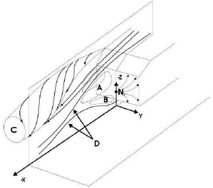
Figure 5: Sketch of vortices and bubble of the time-averaged flow in the near-wake of the Ahmed model.

VI. THE Q-CRITERION

Coherent structures in a turbulent flow are sub-flows with some "cohesive" character, where the turbulence is "self-reorganized" in such a way that the resulting mean motion is rather more regular than chaotic. They have a relatively high concentration of vorticity intensity ω, so they typically show a spiraled motion and they persist for a time scale size τ_c longer than the typical eddy time turnover ω^-1. Previous studies of coherent structures by means of the pressure isosurfaces suggest that a pressure criteria can be better than a vorticity one (Comte et al., 1998). Nevertheless, the threshold value for the pressure isosurfaces shows a strong dependence on the mean pressure around the coherent structures and it can fail in a flow subregion with a high vortex concentration. The so-called Q-criterion (Hunt et al., 1988) is another resource for its study. It is based on both pressure and vorticity intensities and it can be defined as Q = (Ω_ijΩ_ij - S_ijS_ij)⁄2, with Ω_ij = (u_i,j - u_i,j)⁄2 and S_ij = (u_i,j + u_i,j)⁄2, are the symmetrical and skew-symmetrical components of the velocity gradient ∇u respectively. It can be shown that the scalar Q is the second invariant of the velocity gradient ∇u and that it measures the ratio between rotation and deformation rates. Thus, isosurfaces with Q>0 show regions where rotation rates are bigger than the strain ones, so they can develop coherent structures. Since ω²=2Ω², another equivalent definition is Q = (ω² - 2S_ijS_ij)⁄4, showing that the coherent structures have a relatively high concentration of vorticity intensity ω.

VII. NUMERICAL RESULTS

A. Instantaneous flow in the near-wake

A view of the instantaneous flow on the front, top, one lateral side, and partially over the slant surface is shown in the upper plot of Fig. 6, where the flow structure is highlighted through the isosurfaces of the Q-criterion using a threshold of 40 Hz², while at the bottom an experimental observation in a tunnel is included (Beaudoin et al., 2003). The flow pattern is very sensitive to the curvature radii and to the Reynolds number. There are detachments on the curved surfaces at the front part as well as on the intersection between front and top middle surfaces. The transversal Kelvin-Helmholtz vortices are convected downstream from the front side and converted into the hairpin vortices λ, see Fig. 6 (top). The flow separates at the two tilted edges, between the slanted surface and the lateral ones producing two large counter-rotating cone-like trailing vortices. The same figure shows another flow separation on the sharp edge between the body roof and the slant surface, where vortex parallel to the separation line is formed. As it may be observed there is good agreement between numerical and experimental results.

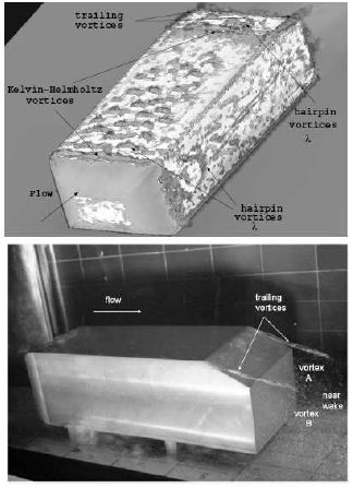
Figure 6: Transversal Kelvin-Helmholtz vortices are downstream convected from the front side and converted into hairpin λ vortices: present computation (top) and experimental of Beaudoin et al. (bottom).

B. Time-averaged flow in the near-wake

The time used for the averaging of the instantaneous flow must be long enough to produce a steady flow. This situation is reached after several hundred of time steps because of stability and accuracy requirements (Krajnović and Davidson, 2004). The symmetry of the time-averaged flow around the vertical symmetrical plane was used as another indicator of the convergence in time of the average flow. The visualizations shown in Figs. 7-11 are all computed through a time-averaged procedure of the large eddy simulations of the unsteady flow, where the averaged-time must be big enough to prevent spurious effects. In this case, the averaged-time is chosen as T = 6T_L where T_L = L⁄U_∞is the elapsed time required by a fluid particle to travel one model length. The visualizations on the body surface are performed by means of trace lines (or friction ones) of the time-averaged flow. The detachments and re-attachments of the time-averaged flow on the body surface are extracted using the Q-criterion. From these numerical results the following features can be observed:

Figure 7: Stream-ribbons of the toroidal horseshoes vortex generated in the separation bubble of the time-averaged flow.

Figure 8: Trace lines of the time-averaged flow showing the singular point N.

Figure 9: A bubble on the slanted surface of the time-averaged flow and some singular points.

Figure 10: Trace lines of the time-averaged flow on the body surface. The flow run left to right.

Figure 11: Trace lines of the time-averaged flow showing singular points on the lateral surface (top-left) and on the slant surface (top-right).

1. In the near-wake there are two large re-circulatory sub-flows A and B situated one over the other which agree with the experimental ones (Ahmed et al., 1984; Gilliéron and Chometon, 1999), see stream-ribbons in Fig. 7. The vortex cores are obtained through a phase plane technique (Kenwright, 1998);

2. The streamlines of the toroidal vortices over the vertical surface produce the singular point N shown in Fig. 8;

3. There is a bubble on the slanted surface shown in Fig. 9, where S₁₀, S₁₁ are half-saddle points while N₆ is a nucleus point;

4. Flow detachments occur on the sharp edges of the model, see Fig. 10. There are three flow detachments on the frontal part: one on the upper side (T) and two more on both lateral sides (L). On the same figure, on both lateral sides, there is a separation zone Z on the top side which encloses the triple border point formed by the front, upper and lateral sides, with a small flow channel due to a high adverse pressure gradient. Also, there is a separation zone L on the middle lateral side;

5. Fig. 11 shows trace lines (or friction ones) of the time-averaged flow showing (i) on the lateral surface (top-left): a center C, a saddle S_s, an unstable focus D and two separation lines; (ii) on the slant surface (top-right): a saddle, a stable focus and a bubble; and (iii) on the top surface (bottom): a saddle, a stable focus, an unstable focus and two separation lines.

C. Topological validation at the symmetrical flow section

A topological validation of the time-averaged flow visualizations is made on the symmetrical section (x = 0) in order to assess if all the main flow structures in the symmetrical section have been identified.

As it is known (Chong et al., 1990), a singular point P in a cut plane ξ, η in a three dimensional flow is a point where velocity vanishes. For its classification, Chong et al. (1990) scheme is adopted here, which is based on the eigenvalues z₁ = a₁ + ib₁ and z₂ = a₂ + ib₂ of the Jacobian matrix H = ∂(u,v)⁄∂(ξ,η) evaluated at the singular point P, where (u,v) are the flow velocities on the cut plane. The resulting taxonomy is summarized in Table 3. It can be noted that in a focus point there is a flow rotation around it as opposed to a node case. Figure 12 shows streamlines as well as singular points of the time-averaged flow that were obtained in the symmetrical section (x = 0), where S₀ to S₁₃ are half saddle points, N₁ to N₇ are focus points (in the vortex nuclei) and D is another saddle point. Figures 13 and 14 show the streamlines projected on the ZY -plane at x = 0. There are half-saddle points S₁,S₂, a focus one N₁ on the top side and the corresponding S₃, S₄ and N₄ on the bottom side. Figure 15 shows the two toroidal vortices F₁ (up per) and F₂ (bottom), whose nucleus are N₄ and N₅, respectively. Figures 16 and 17 show four tiny and small vortices near the vertical surface at the rear end. Two vortices are on the upper region and the remaining two ones on the inferior one. There are vortices whose nucleus B, N₂ and B, N₃ rotate in a clockwise and counter clockwise fashion respectively, and they also have half-saddle points. Near the F₂ vortex a stagnation point P is identified. A bubble formed behind the upper edge of the slanted surface is shown in Fig. 9. On the other hand, on the symmetrical vertical section, the topological relation T = 1 - n must be verified (Hunt et al., 1988), where

; (2)

while is the sum of nodes and focus points, is the sum of the half-node points, is the sum of saddle points, is the sum of half saddle points, and n is the connectivity of the two-dimensional flow section. For instance, the connectivity of any two-dimensional section in a simply connected three dimensional flow region is n = 1 (e.g. a flow without a body) while for the flow around a single body, as in the present case, is n = 2. From the present visualizations, the following values are obtained: = 7, = 0, = 1 and = 14. Therefore T≡1, i.e. the topological restriction is satisfied. It can be concluded that all the main flow structures in the symmetrical section have been identified. These topological features of the time-average flow are found independently of the averaging time T and grid-size of both meshes.

Table 3: A taxonomy for singular points P on a cut plane in a three dimensional flow (Chong et al., 1990).

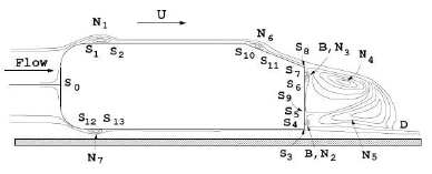
Figure 12: Streamline sketch in a time-averaged sense obtained from the present numerical simulations on the (vertical) symmetry plane x = 0 showing singular points.

Figure 13: Trace lines of the time-averaged flow on the front part at the upper side showing some singular points.

Figure 14: Trace lines of the time-averaged flow on the front part at the bottom side showing some singular points.

Figure 15: Streamlines of the time-averaged flow projected onto the vertical symmetry plane x = 0 showing some singular points.

Figure 16: Tiny vortices of the time-averaged flow on the vertical base surface of the rear end at the upper side B,N₃.

Figure 17: Tiny vortices of the time-averaged flow on the vertical base surface of the rear end at the bottom side B,N₂.

D. Drag and pressure coefficients

The drag coefficient is computed as C_D = D_p⁄γ, with , where D_p is the drag force, A_proy is the frontal surface area, ρ is the fluid density and U_∞ is the non-perturbed speed. The pressure coefficient is defined as , where p_∞is the undisturbed pressure at the inlet boundary. The pressure coefficient for a slant angle α = 12.5° is plotted in Fig. 18 as a function of the streamwise coordinate at the top and bottom body surface on the symmetry plane. In Fig. 19 the unsteady nature of the drag coefficient is shown for the coarser mesh (#1) and the finer one (#2). In each case, oscillations in its values are observed during startup but, after some time-steps, these oscillations become small and approaches a constant value. The mean drag coefficient measured in the wind tunnel tests (Ahmed et al., 1984) for a slant angle of 12.5° was = 0.230 while the numerical are C_D = 0.246 for the coarser mesh, and C_D = 0.228 for the finer one, with a percentage relative error of ε_r%≈ + 6% and ε_r%≈-1%, respectively.

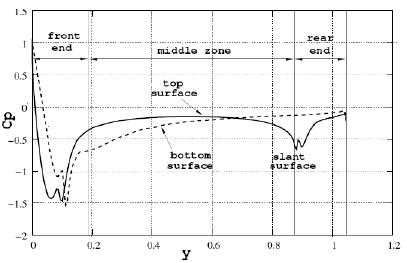
Figure 18: Pressure coefficient C_p as a function of the y-streamwise coordinate at the top and bottom body surface on the symmetry plane for a slant angle a = 12.5°.

Figure 19: Pressure coefficient C_D: time-evolutions, mean values and experimental measured (Ahmet et al., 1984), for a slant angle a = 12.5°.

VIII. CONCLUSIONS

Large Eddy Simulations (LES) with unstructured meshes and finite elements of the unsteady flow around the Ahmed vehicle model were performed for a slant angle of 12.5°. Two meshes were employed, showing mesh convergence through the drag coefficient (see Fig. 19). The symmetry of the time-averaged flow was used as another indicator of the solution convergence. Flow visualizations of the time-averaged flow in the near-wake qualitatively agree with the experimental observations. Most of the features of the flow around this bluff model in ground proximity were predicted, such as the formation of trailing vortices, massive separation and re-circulatory flows. The turbulent eddies up to the Taylor length scale were well resolved. The time-averaged flow was dominated by large coherent macro structures formed by massive flow separation. The mean drag coefficient C_D agrees quite well the experimental one, with a percentual relative error of +6 % for the coarser mesh and -1 % for the finer one. It is found that the topological features of the time-averaged flow are independent of the averaging time T and grid-size. It is concluded that according to the current computational resources LES may be used as a feasible turbulence model for real vehicles aerodynamics. Future modeling efforts would be focused on the representations of the structure of turbulence and some average profiles, as velocities and turbulent stresses, which could be useful for RANS studies.

ACKNOWLEDGMENTS
This work was performed with the Free Software Foundation GNU-Project resources as Linux OS and Octave, as well as other Open Source resources as PETSc, MPICH and OpenDX, and supported through Consejo Nacional de Investigaciones Científicas y Técnicas (CONICET, Argentina, grants PIP-02552/2000, PIP 5271/05) Universidad Nacional del Litoral (UNL, Argentina, grant CAI+D 2005-10-64) and Agencia Nacional de Promoción Científica y Tecnológica (ANPCyT, Argentina, grants PICT 12-14573/2003, PME 209/2003, PICT 1506/2006). N. Calvo has participated in fruitful discussions on mesh quality and mesh generation.

REFERENCES

1. Ahmed, S., G. Ramm and G. Faltin, "Some salient features of the time-averaged ground vehicle wake," SAE Report, 840300, 1-31 (1984).        [ Links ]

2. Barlow, J., R. Guterres, R. Ranzenbach and J. Williams, "Wake structures of rectangular bodies with radiused edges near a plane surface," SAE Congress, 1999-01-0648 (1999).        [ Links ]

3. Basara, B., "Numerical simulation of turbulent wakes around a vehicle," ASME Fluid Engineering Division Summer Meeting, FEDSM99-7324, San Francisco, USA (1999).        [ Links ]

4. Basara, B. and A. Alajbegovic, "Steady state calculations of turbulent flow around Morel body," 7th Int. Symp. of Flow Modelling and Turbulence Measurements, Taiwan, 1-8 (1998).        [ Links ]

5. Basara, B., V. Przulj and P. Tibaut, "On the calculation of external aerodynamics industrial benchmarks," SAE Conf., 01-0701 (2001).        [ Links ]

6. Battaglia, L., J. D'Elía, M. Storti and N.M. Nigro, "Numerical simulation of transient free surface flows," ASME-Journal of Applied Mechanics, 73, 1017-1025 (2006).        [ Links ]

7. Bayraktar, D., D. Landman and O. Baysal, "Experimental and computational investigation of Ahmed body for ground vehicle aerodynamics," SAE Report, 01-2742 (2001).        [ Links ]

8. Beaudoin, J., K. Gosse, O. Cadot, P. Paranthoën, B. Hamelin, M. Tissier, J. Aider, D. Allano, I. Mutabazi, M. Gonzales and J. Wesfreid, "Using cavitation technique to characterize the longitudinal vortices of a simplified road vehicle," Technical report, PSA Peugeot Citroën Directions de la Researche, France (2003).        [ Links ]

9. Beowulf Geronimo cluster, http://www.cimec.org.ar/geronimo (2005).        [ Links ]

10. Calo, V., Residual-based Multiscale TurbulenceModeling: finite volume simulations of bypass transition. Ph.D. thesis, Stanford University (2005).        [ Links ]

11.Calvo N.A., Meshsuite: 3d mesh generation, http://wwww.cimec. org.ar (1997).        [ Links ]

12.Chong, M., A. Perry and B. Cantwell, "A general classification of three-dimensional flow field," Phys. Fluids A, 2, 765-777 (1990).        [ Links ]

13. Comte, P., J. Silvestrini and P. Bégou, "Streamwise vortices in large eddy simulation of mixing layers," Eur. J. Mech, 17, 615-637 (1998).        [ Links ]

14. D'Elía, J., M. Storti and S. Idelsohn, "A panel-Fourier method for free surface methods," ASME-Journal of Fluids Engineering, 122, 309-317 (2000).        [ Links ]

15. D'Elía, J., N. Nigro and M. Storti, "Numerical simulations of axisymmetric inertial waves in a rotating sphere by finite elements," Int. Journal of Computational Fluid Dynamics, 20, 673-685 (2006).        [ Links ]

16. Dubief, Y. and F. Delcayre, "On coherent-vortex identification in turbulence," J. Turbulence, 1, 1-22 (2000).        [ Links ]

17. Duell, E. and A. George, "Experimental study of a ground vehicle body unsteady near wake," SAE Report 1999-01-0812, 197-208 (1999).        [ Links ]

18. ERCOFTAC, European Research Community on Flow, Turbulence and Combustion. http://www.ercoftac.org, (2007).        [ Links ]

19. Garibaldi, J., M. Storti, L. Battaglia and J. D'Elía, "Numerical simulations of the flow around a spinning projectil in subsonic regime," Latin American Applied Research, 38, 241-248 (2008).        [ Links ]

20. Gilliéron, P. and F. Chometon, "Modeling of stationary three-dimensional separated air flows around an Ahmed reference model," ESAIM, 7, 173-182 (1999).        [ Links ]

21. Gilliéron, P. and A. Spohn, "Flow separations generated by a simplified geometry of an automotive vehicle," Technical report, Technocentre Renault - CNRS, Lab. d' Etudes A´erodynamiques de Poitiers (2002).        [ Links ]

22. Han, T., "Computational analysis of three-dimensional turbulent flow around a bluff body in ground proximity," AIIA Journal, 27, 1213-1219 (1989).        [ Links ]

23. Howard, R. and M. Pourquie, "Large eddy simulation of an Ahmed reference model," Journal of Turbulence, 3, 12 (2002).        [ Links ]

24. Hucho, W., Aerodynamics of road vehicles. Society of Automative Engineers (1998).        [ Links ]

25. Hunt, J., A. Wray and P. Moin, "Eddies, stream, and convergence zones in turbulent flows," Report CTRS88, Center For Turbulent Research (1988).        [ Links ]

26.Janssen, L. and W. Hucho, "Aerodynamische Formoptienierung der Typen VW -Golf und VW -Scirocco," Volkswagen Golf I ATZ, 77, 1-5 (1975).        [ Links ]

27. Kapadia, S., S. Roy and K. Wurtzler, "Detached eddy simulation over a reference Ahmed model car," 41st Aerospace Sciences Meeting and Exhibit, AIAA-2003-0857, 1-10 (2003).        [ Links ]

28. Kenwright, D., "Automatic detection of open and closed separation and attachment lines," Proceedings of IEEE Visualization (1998).        [ Links ]

29. Krajnovic, S., Large-Eddy Simulation for computing the flow around vehicles. Ph.D. thesis, Chalmers University of Technology, Sweden (2002).        [ Links ]

30. Krajnovic, S. and L. Davidson, "Numerical study of the flow around the bus-shaped body," ASME-J. of Fluids Engineering, 125, 500-509 (2003).        [ Links ]

31. Krajnovic, S. and L. Davidson, "Large-eddy simulation of the flow around simplified car model," SAE World Congress, Detroit, USA, 2004-01-0227 (2004).        [ Links ]

32. Krajnovic, S. and L. Davidson, "Flow around a simplified car, part 1: Large eddy simulation," Journal of Fluids Engineering, 127, 907-918 (2005a).        [ Links ]

33. Krajnovic, S. and L. Davidson, "Flow around a simplified car, part 2: Understanding the flow," Journal of Fluids Engineering, 127, 919-928 (2005b).        [ Links ]

34. Lienhart, H. and S. Becker, "Flow and turbulence structures in the wake of a simplified car model (Ahmed model)," SAE Report 2003-01(0656) (2003).        [ Links ]

35. McDonough, J., "On intrinsic errors in turbulence models based on Reynolds-Averaged Navier-Stokes equations," Int. J. Fluid Mech. Res., 22, 27-55 (1995).        [ Links ]

36. Message Passing Interface MPI. http://www.mpiforum.org/docs/docs.html (2007).        [ Links ]

37. Morel, T., "Aerodynamics drag of bluff body shapes. characteristics of hatch-back cars," SAE Report, 780267 (1978).        [ Links ]

38.Paz, R. and M. Storti, "An interface strip precondition for domain decomposition methods. application to hidrology," Int. J. for Num. Meth. in Engng., 62, 1873-1894 (2005).         [ Links ]

39. PETSc-2.3.3. http://www.mcs.anl.gov/petsc (2007).        [ Links ]

40. PETSc-FEM. A general purpose, parallel, multi-physics FEM program, GNU General Public License, http://www.cimec.ceride.gov.ar/petscfem (2008).        [ Links ]

41. Sagaut, P., Large eddy simulation for incompressible flows, an introduction. Springer, Berlin (2001).        [ Links ]

42. Sims-Williams, D., "Experimental investigation into unsteadinless and instability in passanger car aerodynamics," SAE Report, 980391 (1998).        [ Links ]

43. Sonzogni, V., A. Yommi, N. Nigro and M. Storti, "A parallel finite element program on a Beowulf Cluster," Advances in Engineering Software, 33, 427-443 (2002).        [ Links ]

44. Spohn, A. and P. Gilliéron, "Flow separations generated by a simplified geometry of an automotive vehicle," IUTAM Symposium: unsteady separated flows. Toulouse, France (2002).        [ Links ]

45. Storti, M.A. and J. D'Elía, "Added mass of an oscillating hemisphere at very-low and very-high frequencies," ASME Journal of Fluids Engineering, 126, 1048-1053 (2004).        [ Links ]

46.Wilcox, D., Turbulence Modeling for CFD. DCW, 2nd edition (1998).        [ Links ]

Received: February 3, 2008
Accepted: August 15, 2008
Recommended by Subject Editor: Eduardo Dvorkin