ARTICLES

Estimation of thermal effusivity of polymers using the thermal impedance method

S. M. M. Lima E Silva¹ and A. L. F. Lima E Silva²

Heat Transfer Laboratory - LabTC, Institute of Mechanical Engineering - IEM, Federal University of Itajubá - UNIFEI,
Itajubá, MG, Brazil.
¹ metrevel@unifei.edu.br,
² alfsilva@unifei.edu.br

Abstract - Thermal impedance is a way of defining the characteristics of thermal systems. It is a function that represents the relation between the frequency components of temperature and heat flux. From the experimental point of view, it is determined simply by measuring the heat flux and the temperature, simultaneously. In this work, these signals are measured only on the frontal surface of the sample. The experimental technique proposed here can be well adapted for making in situ measurements. A one-dimensional semi-infinite thermal model is used. For the semi-infinite model, just the thermal effusivity, b, can be estimated. The thermal effusivity is estimated for three polymers. An objective function representing the difference between experimental and theoretical values of the modulus of the thermal impedance function is minimized. For all cases studied in this work the thermal effusivity is in good agreement with literature. In addition an uncertainty analysis is also presented.

Keywords - Thermal Properties Estimation; Heat Conduction; Optimization; Experimental Methods; Thermal Impedance.

I. INTRODUCTION

Information on thermal transport properties (thermal effusivity, b, thermal conductivity, ? and thermal diffusivity, a) has become increasingly important in a wide range of engineering fields, especially in the evaluation of insulation material performance. In this sense a lot of experimental techniques have been developed for the determination of these properties. These experimental techniques that allow determining the thermal properties values are based upon an identical principle: a signal is produced on the entrance face of a studied material sample, and the thermal response is then recorded at the same face or at another point on the material. This signal is generally an impulse, a periodic function or a step function. Some experimental methods have been used for determining these properties such as the hot wire, flash and photoacoustic methods.

Blackwell (1954) presented the hot wire technique for the measurement of the thermal conductivity. This technique requires inserting a probe inside the sample, and this appears to be the main difficulty of the method when applied to solid materials (it is a destructive method). Another restriction is the use of this method in metallic materials, due to the problems of the contact resistance. Moreover, their high thermal conductivity would greatly reduce the maximum time of measurement. Variations of this method have been used in recent works for the thermal conductivity determination. For example, the ? determination of liquid gallium in Miyamura and Susa (2002) and in Luo et al. (2003) by solving inverse heat conduction problems (IHCP) in an infinite region. Parker et al. (1961) have developed one of the most employed methods for measuring a of solid materials. This method involves exposing a thin slab of the material to a very short pulse of radiant (or other form) energy. The thermal diffusivity is determined through the identification of the time when the rear surface of the sample reaches half of the maximum temperature rise. The use of the flash method to measure a has been employed in countless papers, for instance, in Mardolcar (2002) for rocks at high temperature, in Eriksson et al. (2002) for liquid silicate melts and in Santos et al. (2005) for polymers. However, it should be observed that in the flash method the costs with the experimental apparatus are very expensive. The Photoacoustic method for measuring the thermal effusivity of solids samples based on the theory of layered samples was proposed by Benedetto and Spagnolo (1988). The method consists of the measurement of the phase of the sound pressure generated with a front-surface illumination, as a function of frequency. The sample surface is pained by a black spray whose thermal properties have been previously determined. This allows moreover to eliminate the stray light contribution, which may be important in the case of reflecting samples, as metals with polished surface, and to improve the signal-to-noise ratio, also with low exciting power. Moreover the technique has the advantage of requiring neither laborious sample preparation nor specific ad hoc manufacturing. A possible limit is that the method can not be applied to samples for which the deposition of a surface layer may change the sample properties.

In this work, impulse signals are used in an experimental technique based on the concept of the thermal impedance. The thermal impedance method requires simultaneous measurements of the variations in heat flux and temperature of the measured surface. The sensor, placed on the system to be characterized, induces a disturbance. For a slow change in thermal characteristics and for low frequencies, the disturbance due the sensor is negligible (Defer et al., 1998). The thermal impedance concept has been used in several works (Defer and Duthoit, 1994; Guimarães et al., 1995; Krapez, 2000; Antczak et al., 2003; Jannot and Meukam, 2004; Borges et al., 2006). The estimation of thermophysical properties using thermal impedance method in materials, assumed to be semi-infinite, is very well adapted for making in situ measurements. This method is particularly suitable for studying civil engineering materials. However, for the case of semi-infinite thermal model the medium only depends on its thermal effusivity. In this case, the effusivity is the only parameter that can be identified. It is also possible to determine the thermal conductivity or thermal diffusivity, but one of these values must be known.

The purpose of this paper is to determine the thermal effusivity for three polymers: Polyvinyl chloride (PVC), Polymethyl methacrylate (PMMA) and Polyethylene (PE). For this, a one-dimensional semi-infinite thermal model is used. An objective function representing the difference between experimental and theoretical values of the modulus of the thermal impedance function is minimized to obtain the effusivity. In order to minimize this objective function the optimization technique BFGS is used with the Golden Section technique followed by a polynomial approximation. An error analysis is also conducted to show the improved accuracy of the results of b obtained in the present study. In fact, the method proposed in this work represents an alternate form to estimate b, it can be used for a large range of thicknesses, and there are not restrictions to be adapted for in situ application.

II. THEORETICAL ASPECTS

A. Temperature Model

The thermal model is given by a one-dimensional semi-infinite model as shown in Fig. 1, where f₁ represents the heat flux and ?₁ the upper surface temperature.

Figure 1. Thermal model proposed

The one-dimensional heat diffusion equation for the geometry presented in Fig. 1 can be given by:

(1)

subjected to the following boundary conditions:

(2)

(3)

and the initial condition

(4)

where ?(z,t) = T(z,t) - T₀. In this work, the thermal problem (Eqs. 1-4) is solved in the frequency domain by using the idea of the input/output dynamical system as presented below.

B. Theoretical Thermal Impedance

The technique proposed here uses the input/output dynamical system (Fig. 2), where x and y are the input and output signals, respectively.

Figure 2. Input/output model.

For a semi-finite medium (Fig. 1) the theoretical thermal impedance is given by:

(5)

where b is the thermal effusivity () that is the ability to exchange heat with the environment by the material, f is the frequency and j is the imaginary unit.

C. Experimental Thermal Impedance

By analogy with electrical or mechanical systems, the experimental thermal impedance, Z_e, of a conducting system can be defined in the access plane by the following equation:

(6)

where T₁(f) and F₁(f) represent respectively, the Fourier transforms of ?₁(t) and f₁(t). Z_e(f) is equivalent to the frequency response function and X(f) and Y(f) are the input and output, in the transformed f plane respectively. Their values are found by the application of the Fast Fourier transform of the data x(t) and y(t). The Fourier transforms were performed numerically by using the Cooley-Tukey algorithms (Discrete Fast Fourier Transform) (Bendat and Piersol, 1986). A more stable impedance function can be obtained by multiplying Eq. (6) by the complex conjugate of X(f):

(7)

where S_xy is the cross-spectral density of x(t) and y(t) and S_xx is the autospectral density of x(t).

D. Thermal Effusivity Estimation

The minimization of an objective function, Obj, based on the difference between experimental and calculated values of the modulus of Z is one way to determine the thermal effusivity. This function can be written by:

(8)

where i represents the discrete frequency measurements, nf is the number of frequency measurements used in the optimization process and | Z_e | and | Z | are the experimental and calculated values of the modulus of Z. The sequential unconstrained optimization technique BFGS (Broydon-Fletcher-Goldfarb-Shanno) is used to minimize the objective function (Eq. 8). In addition, the Golden Section method is used in the one­dimensional search, followed by a cubic polynomial interpolation (Vanderplaats, 1984). The package Design Optimization Tools (DOT) (Vanderplaats, 1995) is used to apply the optimization technique.

III. EXPERIMENTAL PROCEDURE

Figure 3 shows the experimental apparatus used to determine the thermal effusivity of polymers materials. Three polymers samples were used: Polyvinyl chloride (PVC), Polymethyl methacrylate (PMMA) and Polyethylene (PE). All the samples have thickness of 50 mm and lateral dimensions of 305 x 305 mm. These lateral dimensions were used in order to guarantee that the sample could be submitted to a unidirectional and uniform heat flux on its upper surface, where at time t = 0 s (T₀), the sample is in thermal equilibrium. The heat is supplied by a 22 O electrical resistance heater, covered with silicone rubber, with lateral dimensions of 305 x 305 mm and with 1.4 mm of thickness.

Figure 3. Scheme of the experimental apparatus.

A heat flux transducer with lateral dimensions of 50 x 50 mm, thickness of 0.1 mm, and constant time less than 10 ms measures the heat flux input (Leclerq and Thery, 1983). The transducer is based on the thermopile conception of multiple thermoelectric junction (made by electrolytic deposition) on a thin conductor sheet. The electromotive force (emf) measured is proportional to the heat flux crossing the measured area. The evolution of temperature with time at the upper frontal boundary surface is measured using a K type cable thermocouple (40 AWG). These sensors were placed under pressure with a thermal grease to reduce the contact resistance. The signals of temperature and heat flux are acquired by a data acquisition system HP Series 75000 with a voltmeter E1326B controlled by a personal computer.

IV. DEFINITION OF THE EXPERIMENTAL PARAMETERS

A. Comparison of Thermal Models

As already mentioned, the semi-infinite model must be used for the determination of b. In this work, the used samples are finites with a thickness of L = 50 mm. However, under certain conditions of time the thermal behavior of a finite medium of thickness L can be considered identical to the semi-infinite medium (Beck et al., 1992). In addition, this behavior tends to be the same as larger the thickness of the medium and smaller the time of heat diffusion. In order to verify this condition, a comparison between a finite model and a semi-infinite model is done for the calculated temperatures on the frontal surface (Figure 4a).

	(a)
	(b)
Figure 4. a) Comparison of the temperature evolution for the finite and semi-infinite models b) Residuals of temperature.

The used finite model is a one-dimensional model with heat flux imposed on the frontal surface and isolated on the other surface. In this case, the signal of heat flux supplied to each one of the samples, studied in this work, is used for the calculation of these temperatures. Figure 4a presents this comparison for the sample of PVC. For this study the values of thermal properties a = 1.28 x 10^-7 m²/s and ? = 0.156 Wm/K from Lima a Silva et al. (2003) were used. However, a small discrepancy occurs, it can be noted that the residuals presented in Fig. 4b are situated in the range of uncertainty measurement of thermocouples, which in this work is ± 0.3 K. Another important analysis of the semi-infinite condition can be found in Antczak et al. (2003). These authors mentioned that to justify this condition the thickness of the sample must be larger or equal to 3e, with . This condition was also verified. Thus, the use of the semi-infinite thermal model is guaranteed. The same results were obtained for the PMMA and PE samples.

B. Sensitivity Analysis

Another important way of analysis is to study the behavior of the sensitivity coefficient involved in the process. The analyzed sensitivity coefficient S_b is defined as the first derivative of the modulus of Z with respect to the parameter b. Figure 5 shows the behavior of S_b in the frequency domain for each sample. It can be seen that for frequencies greater than 2.0 x 10^­3 Hz, S_b becomes constant and a little contribution is given to the estimation procedure for all cases. Besides, in Fig. 6 the real component of the cross-spectral density calculated for PVC is presented. This figure also shows that for frequencies higher than 0.002 Hz a little change happens. In this case the same number of points obtained by the sensitivity coefficient is used to estimate b. The same behavior is presented for PMMA and PE. In this case, fourteen points for PVC, nine points for PMMA and fourteen points for PE were used to determine b.

Figure 5. Sensitivity coefficients related to PVC, PMMA and PE

Figure 6. Real component of the cross-spectral density

V. RESULTS

Fifty independent runs for PVC, forty for PMMA and twenty for PE were carried out. The number of points used for each sample was 8192 for PVC, 4096 for PMMA and 1024 for PE. The time steps, ?t, were 0.8793s for PVC, 1s for PMMA and 6.242s for PE. The difference among the procedures is because the data were obtained from three different works. For PE (Guimarães et al., 1995), PMMA (Lima a Silva et al., 1998) and PVC (Lima a Silva et al., 2003). As the equipments are the same these experiments were used in the present work. It is important to mention that some conditions are necessary when the frequency domain is used. For the number of points a power of 2 (two) and a great quantity of points must be used. In addition, the time steps have to be small to have a better band to work in frequency domain. The global time of heating, t_h, for PVC and PMMA was approximately 150s and for PE it was approximately 90s. The generated heat pulse was 40 V (dc) supplied for the three materials. Figures 7a and 7b present, respectively, the heat flux and temperature signals in the upper surface of the PVC sample. As the heat flux and temperature curves for the PMMA and PE samples have the same behavior of the PVC, these curves are presented only for PVC sample. In Figure 8a a comparison between estimated and experimental modulus of the impedance function for PVC is presented. It can be observed a very good agreement. Figure 8b shows the residuals. The same agreement presented in Fig. 8b was found for the samples of PMMA and PE. Figures 9 to 11 present the values obtained for b for all samples studied.

	(a)
	(b)
Figure 7. a) Evolution of the input signal x(t) = f1(t) b) Evolution of the output signal y(t) = ?1(t)

	(a)
	(b)
Figure 8. a) Experimental and calculated modulus of Z b) Residuals of | Z |

Figure 9. Histogram of b for PVC

Figure 10. Histogram of b for PMMA

Figure 11. Histogram of b for PE

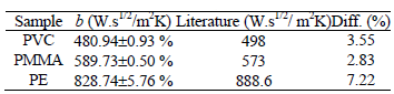
When analyzing a series of measurements some data can present uncertainties that interfere in the process, causing inexact values (Taylor, 1997). The experiments for each sample were repeated many times in order to reduce these uncertainties, as presented in Figs. 8 to 10. Thus, the value of b found for each sample is an average of the values presented in Figs. 8 to 10. Table 1 presents the estimated mean value and standard deviation of b for the three samples studied. This mean value of b was obtained using a confidence interval of 99.7 %. In this table, the values of b from literature were obtained from Defer et al. (2001), for PVC, from Gustavsson et al. (2005) for PMMA and from Jannot and Meukam (2004) for PE. It can be observed that the results presented good agreement with the respective reference values.

Table 1. Statistic data to the average values estimated for b.

VI. UNCERTAINTY ANALYSIS

A. Introduction

For the determination of b with accuracy, the errors must be minimized (Taylor, 1997). The causes of these errors are many. In the case of thermal properties determination, the most common ones are: errors in the restrictions of the theoretical model, errors in temperature and heat flux measurements due to calibration, time response and thermal contact resistance in the sensors and the measurement uncertainty in the data acquisition of the signals. In addition, numerical errors can also be produced when calculating the distributions and using the Fast Fourier Transform and they must be taken into account.

B. Uncertainty Analysis in the Determination of b

The used procedure for the estimation of error in the determination of b is based on the propagation calculus of the uncertainties in the measurement of the original variables (heat flux and temperature) and the numerical calculus of the Fast Fourier Transform in these signals. Once the objective function, Obj, is based on the difference between experimental and calculated values of the modulus of Z, in this work the hypothesis of linear propagation is used. The hypothesis of one-dimensional heat flux is qualitatively analyzed through the numerical simulation. The results of the simulation assure the hypothesis of one-directional heat flux. These simulations were done inside the experimental conditions used in this work as: materials of low conductivity (polymers), sample with dimensions of 305 x 305 x 50 mm and the total time of heating of approximately 150 s for the three samples (Lima a Silva, 2000). Bias errors due to the thermal contact between the sensors and samples were analyzed by Guimarães (1993). The results obtained by Guimarães (1993) assure the hypothesis of perfect thermal contact between the sensors and the sample. In this sense, the measurement uncertainty in the original variables is estimated as the partial uncertainties in the data acquisition system and in the calibration of the temperature and heat flux sensors. From the theory of linear propagation errors (Taylor, 1997), the uncertainty of the temperature can be calculated from the uncertainties of the data acquisition system and temperature sensor (thermocouple) as:

(9)

Also from the theory of linear propagation errors, the uncertainty of the heat flux is obtained from the uncertainties of the data acquisition system and heat flux sensor (heat transducer) as:

(10)

Thus, the uncertainty in the objective function Obj can be obtained through the analysis of the uncertainty propagation in the temperature (Eq. 9), in the heat flux (Eq. 10) and in the numerical errors produced when using the Fast Fourier Transform. The calculus of the FFT is done over temperature and heat flux. In this case the uncertainty in the Obj can be given by:

(11)

The used data acquisition is a Data Acquisition/Control HP 75000 produced by Hewlett Packard with a voltmeter E1326B controlled by a personal computer. Excepting the relative uncertainty to the sensors, all the other elements of measurement, as the voltmeter, cables and functional modules, operating in the range of temperature between 20 and 35 °C, auto-zero on with NPLC = 1, range of 125 mV and with warm-up of one hour, have an uncertainty estimated in:

(12)

The thermocouple uncertainty can be obtained from the uncertainty of the temperature controller bath (Thermometry Calibration System) manufactured by ERTCO, with maximum fluctuation of ± 0.1 °C and mean temperature of 30.5 °C by:

(13)

The uncertainty of the heat transducer can be estimated from the previous calibration, considering the uncertainties in the tension, current and area of measurement, that is:

(14)

The uncertainty in the Fast Fourier Transform is obtained from the comparison of the calculated temperatures numerically (using FFT) with analytically (Lima a Silva et al., 1998) and was estimated in:

(15)

For the objective function of impedance the uncertainty was obtained by substituting Eqs. (12-15) in Eq. (11) as:

(16)

Thus, from the hypothesis of linear propagation of errors, the uncertainty in the estimated thermal effusivity is given by:

(17)

It can be observed that the estimated value for the uncertainty of b is conservative. In some cases as in the determination of the difference of experimental temperature, the random errors of measurement tend to compensate reciprocally. This fact also contributes for a lower real uncertainty for the calibration of the heat transducer. However, the uncertainty presented in this work should only serve as a reference value. Some aspects, as the possible current leakage in the calibration of the heat flux transducer were not analyzed. In addition the influence of the time response in the heat flux transducer and thermocouple (less than 0.01 s) was also despised. It can be observed that the sampling interval of the signals were of 0.879 s for PVC, 1.0 s for PMMA and 6.243 for PE. In spite of this, the values of b obtained for PVC, PMMA and PE are placed inside the band of uncertainty specified for the reference values. These results indicate that the estimated uncertainty for the analyses presented above is sufficiently representative.

VII. CONCLUSIONS

This work showed that thermal impedance could be used as a means of non-destructive testing and that it provides quantitative information on a conductive system. The experimental procedure is very simple with inexpensive devices used for the measurements. It is easy to implement and involves simply placing sensors of temperature and heat flux on the surface of the material. The thermal effusivity results are in good agreement with literature. For all the cases studied the difference is less than 3.6 % for PVC and PMMA. In the case of PE the difference is higher because the number of experiments used was only 1024. This technique can also be used for applications to conducting materials.

AKNOWLEDGMENTS
The authors would like to thank CNPq, FAPEMIG and CAPES, government agencies for the financial support without which this work would not be possible. They are also grateful to Prof. Gilmar Guimarães for the technical support and for the experimental data of Polyethylene.

REFERENCES

1. Antczak, E., A. Chauchois, D. Defer and B. Duthoit, "Characterization of the thermal effusivity of a partially saturated soil by the inverse method in the frequency domain," Applied Thermal Engineering, 23, 1525-1536 (2003).        [ Links ]

2. Beck, J.V., K.D. Cole, A. Haji-Sheikh and B. Litkouhi, Heat Conduction Using Green's Functions, Hemisphere Publishing Corporation, Washington D.C (1992).        [ Links ]

3. Bendat, J.S. and A.G. Piersol, Analysis and Measurement Procedures, Wiley­Intersience, 2° Ed., USA (1986).        [ Links ]

4. Benedetto, G. and R. Spagnolo, "Photoacoustic measurement of the thermal effusivity of solids," Applied Physics A - Materials Science & Processing, 46, 169-172 (1988).        [ Links ]

5. Blackwell, J.H., "Transient-flow method for determination of thermal constants for insulating materials in bulk," Journal of Applied Physics, 25, 137-144 (1954).        [ Links ]

6. Borges, V.L., S.M.M. Lima e Silva and G. Guimarães, "A Dynamic thermal identification method applied to conductor and non conductor materials," Inverse Problems in Science and Engineering, 14, 511-527 (2006).        [ Links ]

7. Defer, D. and B. Duthoit, "Caractérisation thermique sous sollicitations aléatoires. notion d'impedance thermique appliquée aux mesures in situ," Rev. Gén. Thermique, 33, 633-640 (1994).        [ Links ]

8. Defer, D., E. Antczak and B. Duthoit, "The characterization of thermophysical properties by thermal impedance measurements taken under random stimuli taking sensor-induced disturbance into account," Meas. Sci. Technol., 9, 496-504 (1998).         [ Links ]

9. Defer, D., E. Antczak and B. Duthoit, "Measurement of low thermal effusivity of building materials using the thermal impedance method," Meas. Sci. Technol., 12, 549-556 (2001).         [ Links ]

10. Eriksson, R., M. Hayashi and S. Seetharaman, "Thermal Diffusivity Measurements of Liquid Silicate Melts," Proc. The Sixteenth European Conference for Thermophysical Properties (ECTP2002), London, UK (2002).        [ Links ]

11. Guimarães, G., Estimação de Parâmetros no Domínio da Frequência para a Determinação Simultânea da Condutividade Térmica e Difusividade Térmica, Doctoral Thesis, (in Portuguese), Universidade Federal de Santa Catarina, Brazil (1993).         [ Links ]

12. Guimarães, G., P.C. Philippi and P. Thery, "Use of parameters estimation method in the frequency domain for the simultaneous estimation of thermal diffusivity and conductivity," Review of Scientific Instruments, 66, 2582-2588 (1995).         [ Links ]

13. Gustavsson, M., H. Nagai and T. Okutani, "Measurements of the thermal effusivity of a drop-size liquid using the pulse transient hot-strip techniques," International Journal of Thermophysics, 26, 1803-1813 (2005).        [ Links ]

14. Jannot, Y. and P. Meukam, "Simplified estimation method for the determination of the thermal effusivity and thermal conductivity using a low cost hot trip," Meas. Sci. Technol, 15, 1932-1938 (2004).        [ Links ]

15. Krapez, J.C., "Thermal effusivity profile characterization from pulse photothermal data," Journal of Applied Physics, 87, 4514-4524 (2000).        [ Links ]

16. Leclerq, D. and P. Thery, "Apparatus for simultaneous temperature and heat-flow measurements under transient conditions," Review of Scientific Instruments, 54, 374-380 (1983).        [ Links ]

17. Lima e Silva, S.M.M, M.A.V. Duarte, and G. Guimarães, "A Correlation Function for Thermal Porperties Estimation Applied to a Large Thickness Sample with a Single Surface Sensor," Review Scientific Instrument, 69, 3290-3297 (1998).        [ Links ]

18. Lima e Silva, S.M.M., Experimental techniques development for determining thermal diffusivity and thermal conductivity of non-metallic materials using only one active surface, Doctoral Thesis, (in Portuguese), Federal University of Uberlândia, Brazil (2000).        [ Links ]

19. Lima e Silva, S.M.M., T.H. Ong and G. Guimarães, "Thermal properties estimation of polymers using only one active surface," J. of the Braz. Soc. Mechanical Sciences, 25, 9-14 (2003).        [ Links ]

20. Luo, D., L. He, S. Lin, T.F. Chen and D. Gao, "Determination of temperature dependent thermal conductivity by solving IHCP in infinite region," Int. Comm. Heat Mass Transfer, 30, 903-908 (2003).        [ Links ]

21. Mardolcar, U.V., "Thermal diffusivity of rocks at high temperature by the laser flash technique," Proc. The Sixteenth European Conference for Thermophysical Properties (ECTP2002), London, UK, (2002).        [ Links ]

22. Miyamura, A. and M. Susa, "Relative measurements of thermal conductivity of liquid gallium by transient hot wire method," Proc. The Sixteenth European Conference for Thermophysical Properties (ECTP2002), London, UK, (2002).        [ Links ]

23. Parker, W.J., R.J. Jenkins, C.P. Butler and G.L. Abbott, "Flash method of determining thermal diffusivity, heat capacity and thermal conductivity," Journal of Applied Physics, 32, 1679-1684 (1961).        [ Links ]

24. Santos, W.N., P. Mummery and A. Wallwork, "Thermal diffusivity of polymers by the laser flash technique," Polymer Testing, 24, 628-634 (2005).         [ Links ]

25. Taylor, J.R., An Introduction to Error Analysis: The Study of Uncertainties in Physical Measurements, University Science Books, 2^nd ed., (1997).         [ Links ]

26. Vanderplaats, G.N., Numerical Optimization Techniques for Engineering Design, McGraw-Hill Inc. (1984).        [ Links ]

27. Vanderplaats G.N., Design Optimization Tools, Vanderplaats Research & Development", Inc., Colorado Springs (1995).         [ Links ]

Received: July 14, 2008.
Accepted: March 17, 2009.
Recommended by Subject Editor Walter Ambrosini.