ARTICLES

Identification of biochemical reactors using fractional differential equations

L. A. D. Isfer¹, M. K. Lenzi¹ and E. K. Lenzi²

¹ Dpto de Eng. Química, Univ. Fed. do Paraná, Jardim das Américas, CP 19011, Curitiba-PR, 81531-990, Brazil
lenzi@ufpr.br
² Dpto de Física, Univ. Est. de Maringá, Avenida Colombo 5790, Maringá-PR, 87020-900, Brazil
eklenzi@dfi.uem.br

Abstract — High production meeting product quality, process safety and environmental regulation provide to control systems a key role in biochemical plants operation. As a suitable mathematical model is essential for process control, this work reports an alternative tool, based on the use of fractional order differential equations, for biochemical reactor identification using previously reported experimental data. Three different approaches were considered: i) solving the nonlinear set of algebraic equations obtained from the derivatives of the objective function with respect to the parameters; ii) solving a multivariable nonlinear deterministic optimization problem; iii) solving a multivariable nonlinear heuristic optimization problem. All identified models were submitted to statistical fitting tests and the second approach (ii) proved to be the most efficient for process identification, satisfying all statistical tests. Common integer order models were identified, leading to poorer data fit when compared to the fractional model, proving the usefulness and success identification tool proposed.

Keywords — Process Identification; Fractional Differential Equation; Caputo Representation; Biochemical Reactor.

I. INTRODUCTION

Due to the needs of high production meeting product quality, process safety and environmental regulation, control systems play a key role in chemical and biochemical plants operation (Santos et al., 2005). However, in order to have a well regulated system, a suitable and reliable mathematical model must be available. First principle models are usually better than empirical models not only because of the theoretical background, but also due to the extrapolation capability allowed by proper parameter estimation (Levenspiel, 2002). On the other hand, fundamental models may be too large for real time application, besides, some difficulties may arise during the modeling task, such as the choice of constitutive relations for example the kinetic equation or thermodynamic equation of state (Lenzi et al., 2005). A commonly used alternative employed to overcome these difficulties is the use of empirical models, which can be obtained by process identification techniques (Pearson, 2006). Modeling and identification of biochemical reactors represent a broad research field with several successful applications already reported in literature. Results concern fundamental and empirical modeling (Kirdar et al., 2008), applications to membrane reactors (Ng and Kim, 2007), solid-state fermentation (Mitchell et al., 2004), gas-lift reactors (Petersen and Margaritis, 2001).

Fractional differential order equations represent a fast growing research field (Hilfer, 2000). Different applications of fractional calculus have been reported ranging from diffusion studies (Lenzi et al., 2006) to stock market applications (Bianco and Grigolini, 2007), while other important applications such as in rheological behavior are also reported (Craiem et al., 2008). Further details regarding the formalism of fractional calculus (Oldham and Spanier, 2006) and the physical interpretation of fractional derivatives (Machado, 2003) are beyond the scope of this work and can be found elsewhere. Successful results concerning fractional identification have reported by Poinot and Trigeassou (2004). The authors report an output-error technique for fractional identification. The reported results indicate that good models can be obtained however the identification technique is a hard task, as it is divided into three steps, one for steady state gain estimation, a second for the system time constant estimation and finally the order of the derivate. Another approach is reported by Hartley and Lorenzo (2003) where frequency analysis is used for system identification.

This work reports an alternative tool for biochemical reactors identification, which was validated with experimental data reported in the literature (Isfer, 2009). To our knowledge, fractional differential equations have not been yet used for modeling or identification of biochemical reactors using actual experimental data. The aim of this work is not only the process identification, but also the analysis of different parameter estimation approaches used with fractional differential equations. The different approaches considered for parameter estimation step involved in the identification task were: i) solving a nonlinear set of algebraic equations, obtained from de derivatives of the objective function with respect to the parameters being estimated; ii) solving a multivariable nonlinear deterministic optimization problem; iii) solving a multivariable nonlinear heuristic optimization problem, based on genetic algorithms. These techniques were used not only for fractional identification, but also for first and second integer order models. After parameter estimation, the identified models are analyzed by standard statistical tests (Otto, 1999) in order to quantify and evaluate the quality of the achieved data fitness.

II. THEORETICAL FRAMEWORK

A fractional derivate can be obtained by several approaches (Isfer, 2009). However, in this work, only the Caputo representation (Caputo, 1967), presented bellow, will be considered.

(1)

where: m < ß < m+1; ß ∈ ℜ; m ∈ ℵ

The main advantages of this representation are the fact that initial conditions of the fractional differential equations can be expressed in terms of integer order derivatives (Hilfer, 2000). Secondly, for this representation, the fractional derivate of a constant function is zero allowing the use of deviation variables (Seborg et al., 2003), which considerably simplify the mathematical analysis when using Laplace transform. In this work the following transfer function (Laplace domain) is used for biochemical reactor identification. In this model, a is the order of the derivate. It can be observed that when a=1 or a=2 Eq. (2) represents first and second order transfer functions, respectively. Due to the memory effect feature of the fractional derivate, systems exhibiting nonlinear behavior can also be identified by the transfer function.

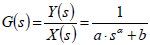(2)

If X(s) is a unit step (Heaviside Function), which is a common disturb used for process identification, the behavior of Y(s) in time domain is given by Eq. (3), which was obtained by Laplace inversion. Further details of the algebraic operation can be found in Lenzi et al. (2006).

(3)

III. METHODOLOGY

The objective function used for parameters a, b, a estimation is given bellow, where NE is the number of experiments and y_OBS-p is the observed experimental value at instant p.

(4)

According to Bard (1974), the parameter estimation task can be carried out using two different approaches: i) solving a nonlinear set of algebraic equations, obtained from de derivatives of the objective function with respect to the parameters being estimated; ii) solving a multivariable nonlinear optimization problem, which can be done by using either a deterministic or a heuristic optimization method.

The first approach consists in solving the set of non-linear of algebraic equations given by Eq. (5) to Eq. (8).

(5)

According to Lebedev (1972), Ψ function can be used for evaluation of gamma function derivate.

	(6)
	(7)
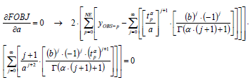	(8)

This set of equations was solved using a modified Powell algorithm (Himmelblau and Edgar, 2002), which considered a finite difference based approximation for Jacobian matrix calculation. The evaluation of gamma (?) and Ψ functions was carried out using numerical integration through quadratures with 20 collocation points (Rice and Do, 1995). The series with upper limit equal to ∞ was considered completely evaluated when the last calculated term was less than 10^-70.

The second approach used for parameter estimation was the solution of a nonlinear multivariate optimization problem using a deterministic technique. In this work, a quasi-Newton method (Himmelblau and Edgar, 2002), with a finite-difference based approximation for the gradient vector was used for parameter estimation. Finally, a third approach considered a heuristic technique for solving the optimization problem. Due to facility of implementation and convergence issues, genetic algorithm strategy was chosen (Himmelblau and Edgar, 2002). Simulations were carried out using 20 genes and 150 generations, where each gene is formed by a set of parameters {a,b, a}. The number of genes and generations were chosen according to Ahn (2006) guidelines, assuring that the simulations are fast enough and also lead to consistent results. Following the guidelines, crossover and mutation probabilities were of 80% assuring a good macroscopic search and of 10% assuring a good microscopic (refinement), respectively.

In this work three different models were used for reactor identification and each model was identified by the three approaches previously described, resulting in nine different identified models. All models are based on Eq. (2). Model 01 is formed by Eq. 1 where a is set equal to 1 (integer). Model 02 is formed by Eq. 1 where a is set free, considered a real number. Model 03 is formed by Eq. 3 where a is set equal to 2 (integer). Model 02 is a fractional order model, while Model 01 and Model 03 are integer order models, which were identified as a benchmark for comparison. After parameter estimation, statistical tests were performed to evaluate the good of fitness. Particularly, the calculation of correlation coefficient, mean and variance hypothesis tests and Chi-square (χ²) test were carried out (Otto, 1999). These are standard statistical tests and details regarding their implementation can be found elsewhere (Johnson and Wichern, 2002). Finally, parameter variance should be also estimated in order to verify parameter significance. In this work, parameter variation was obtained according standard procedures reported by Bard (1974).

The experimental data set used is reported Isfer (2009), and describes the behavior of the concentration of CO₂ of a bioreactor after a step change in the feed flow rate to this reactor. The experimental points are from yeast alcoholic fermentation, described by the following reaction: C₆H₁₂O₆ → 2(CH₃CH₂OH) + 2(CO₂). The experimental variance is reported to be equal to 1.5·10^-4 constant and equal for all data values. A small value of variance was chosen to give consistency and reliability to the experimental data. Secondly, if higher variance values are used, larger vertical bars have to be used for experimental data representation, allowing two or more distinct models to fit the data from a statistical point of view, as the model predictions would lay in the confidence interval. Finally, a constant and equal value of variance can be assumed when random errors are lower than the smallest value of the scale used for the measurement (See Fig. 1).

IV. RESULTS AND DISCUSSIONS

In this section, results concerning parameter estimation and statistical tests will be presented and discussed. Table 1 presents the results regarding parameter estimates for Model 01, Model 02 and Model 03 for the three approaches.

Table 1 - Parameter Estimation Results

Besides, the best obtained parameter estimates; Table 1 also reports the values of the objective function (Eq. 4) for each set of parameters estimates. The initial guesses were randomly chosen. One can observe that, independently of the approach used for parameter estimation, Model 02 is the best if the value of FOBJ is the considered criterion. It can be observed that the value of FOBJ is one order of magnitude lower than the values obtained for Model 01 and Model 03. The second approach led to better parameter estimates taking into account the value of FOBJ. If Approach 02 is compared to Approach 03, this probably happened due to the use of gradients of the objective function to guide the search towards the minimum, as in Approach 02 a deterministic optimization method was used. On the other hand, it should be kept in mind that the choice of the initial guesses in Approach 02 plays a crucial role for parameter estimation. So, it is possible to infer that the results of Approach 03 may represent good initial guesses for Approach 02, due to the large number of initial guesses used in Approach 03. If Approach 02 is compared to Approach 01 the difference probably happened because of the choice of the solver used to obtain the solution of the set of non-linear equations. Figure 1 presents model prediction values for the three models and experimental data plotted against time.

Figure 1 - Model predictions and experimental data against time - Approach 02

It can be observed that with the exception of the first point, all predictions of Model 02 lie within the confidence interval of the experimental point which is represented by the vertical bar error.

However, despite the qualitative fitness observed, in Fig. 1, two other important plots should be analyzed. The first is shown in Fig. 2 where model predicted values are plotted against experimental values. If the model is perfect, data should lie over the straight line presented. It can be observed that for Model 02 predicted values are close to experimental data and are randomly distributed over the straight line; differently situation happens to Model 01 and Model 03 predictions.

Figure 2 - Model predictions against experimental data - Approach 02

An important plot is reported by Fig. 3, where the residues between experimental values and model predictions are plotted in a vertical bar chart. A reliable conclusion from this figure is that besides being close to zero, the residues of Model 2 are randomly distributed over zero. This indicates that the difference between experimental and predicted values occurs due to random experimental error allowing one to conclude that no systematic error or bias is present. For Model 03, the residues are too large, while for Model 01, a linear tendency of the residues can be observed at the initial points.

Figure 3 - Residues between Model predictions and experimental data against time - Approach 02

Statistical tests are also important to evaluate the identified models, which were obtained after the parameter estimation tasks. Table 2 reports the results of the correlation coefficient calculation performed according to Johnson and Wichern (2002). It can be observed that the R value of Model 02 is the closest to 1 evidencing a good fit. However, it should be mentioned that Model 01 also led to R close to 1. This probably happened because the model data have the experimental data tendency leading to a good value of R despite the residue, which mainly influences the value of FOBJ.

Table 2 - Correlation coefficient results

Another important statistical test which can be used is reported by Otto (1999). It is a mean and variance hypothesis tests which were performed between the experimental data set and each model prediction data set. Table 3 presents the obtained results. The value of F_THEORETICAL is obtained from the Fischer distribution considering the level of confidence and the degree of freedom of each case and is used for a variance hypothesis test. On the other hand, the value of t_THEORETICAL is obtained from t-student distribution considering the level of confidence and the degree of freedom of each case and is used for the mean hypothesis test. Afterwards, a mean hypothesis test is conducted. From the reported results one can infer that the experimental data set and the data sets formed by model the three models predictions are the same considering 99% of confidence level.

Table 3 - Mean and variance hypothesis tests results

A third and important test is reported bellow. This test of goodness of fit is reported by Otto (1999) and takes into account the individual variance of the experimental data which was considered constant and equal to 1.5·10^-4. It will also be considered a confidence level of 99%. Table 4 lists the obtained results. The values of lower and upper were obtained from the Chi-square distribution using the degree of freedom and confidence level according to the analyzed case. It can be observed that only the fractional model satisfied this test. It is important to stress the importance of performing all statistical tests and do not rely only on the R value. Finally, it is important to realize that the results of this test are in agreement with the qualitative analysis involving the residual plots. It is also worth mentioning that one may choose an experimental variance higher than to 1.5·10^-4 in order to satisfy all criteria. However, higher values reduce the reliability of the experimental data and also the model likelihood.

Table 4 - Test of goodness of fit

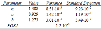
Finally, Table 5 reports the parameter variance obtained using the reported techniques by Bard (1974), where the objective function was linearized in the region close to the parameter estimate values. It can be observed that both variance and standard deviation are much smaller than the parameter value itself, allowing the conclusion that the parameters and their effects are significant. From the reported results, for the experimental data set used only the identified fractional model satisfied all statistical tests.

Table 5 - Parameter variance

V. CONCLUSIONS

An experimental data set previously reported in the literature was used for fractional identification through three different approaches: i) solving a nonlinear set of algebraic equations, obtained from de derivatives of the objective function with respect the parameters to be estimated; ii) solving a multivariable nonlinear deterministic optimization problem; iii) solving a multivariable nonlinear heuristic optimization problem, based on genetic algorithms. The second approach (ii) proved to be the most efficient for process identification, leading to a fractional model that not only has correlation coefficient of roughly 0.999, but also satisfies all statistical tests considered. Predicted and experimental data plots were used for qualitative analysis of the identification. Experimental data were also identified by common first and second order models, which led to a poorer data fit when compared to the fractional model, proving the usefulness and success of fractional identification tool proposed.

VI. ACKNOWLEDGEMENTS
The authors are thanked to CNPq, Fundação Araucária and PRH24/ANP (Brazilian Agencies) for providing financial support for this project.

REFERENCES

1. Ahn, W.C. Advances in Evolutionary Algorithms-Theory, Design and Practice, Springer-Verlag, Berlin (2006).        [ Links ]

2. Bard, Y., Nonlinear Parameter Estimation, Academic Press, New York (1974).        [ Links ]

3. Bianco, S. and P. Grigolini, "Aging in financial market", Chaos Soliton Fract., 34, 41-50 (2007)        [ Links ]

4. Caputo, M. "Linear model of dissipation whose q is almost frequency independent - II", Geophys. J. R. Astr. Soc., 13, 529-539 (1967).        [ Links ]

5. Craiem, D.O., F.J. Rojo, J.M. Atienza, G.V. Guinea and R.L. Armentano, "Fractional Calculus Applied To Model Arterial Viscoelasticity", Latin Am. Appl. Res., 38, 141-145 (2008).        [ Links ]

6. Hartley, T.T. and C.F. Lorenzo, "Fractional-order system identification based on continuous order-distributions", Signal Process., 83, 2287-2300 (2003).        [ Links ]

7. Hilfer, R., Applications of Fractional Calculus in Physics, World Scientific, Singapore (2000).        [ Links ]

8. Himmelblau, D.M. and T.F. Edgar, Optimization of Chemical Processes, Mcgraw-Hill, New York, (2002).        [ Links ]

9. Isfer, L.A.D., Fractional identification and control of chemical systems (In Portuguese), Msc. Thesis, Federal University of Parana (2009).        [ Links ]

10. Johnson, R.A. and D.W. Wichern, Applied Multivariate Statistical Analysis, Prentice-Hall, Upper Saddle River (2002).        [ Links ]

11. Kirdar, A.O., K.D. Green and A.S. Rathore, "Application of multivariate data analysis for identification and successful resolution of a root cause for a bioprocessing application", Biotechnol. Prog., 24, 720-726 (2008).        [ Links ]

12. Lebedev, N.N., Special Functions and Their Applications, Dover Publications, New York (1972).        [ Links ]

13. Lenzi, M.K., M.F. Cunningham, E.L. Lima and J.C. Pinto, "Modeling of semibatch styrene suspension polymerization processes", J. Appl. Polym. Sci., 96, 1950-1967 (2005).        [ Links ]

14. Lenzi, E.K.; M.K. Lenzi, R.S. Mendes, G Goncalves and L.R. Silva, "Fractional diffusion equation and green function approach: exact solutions", Phys. A. 360, 215-226 (2006).        [ Links ]

15. Levenspiel, O., "Modeling in chemical engineering", Chem. Eng. Sci., 57, 4691-4696 (2002).        [ Links ]

16. Machado, J.A.T. "A probabilistic interpretation of the fractional-order differentiation", Fract. Calc. App. Analys. 6, 73-80 (2003).        [ Links ]

17. Mitchell, D.A., O.F. Von Meien, N. Krieger and F.D.H. Dalsenter, "A review of recent developments in modeling of microbial growth kinetics and intraparticle phenomena in solid-state fermentation", Biochem. Eng. J., 17, 15-26 (2004).        [ Links ]

18. Ng, A.N.L. and A.S. Kim, "A mini-review of modeling studies on membrane bioreactor (MBR) treatment for municipal wastewaters", Desalination, 212, 261-281 (2007).        [ Links ]

19. Oldham, K.B. and J. Spanier, The Fractional Calculus, Dover Publications, New York (2006).        [ Links ]

20. Otto, M., Chemometrics: Statistics and Computer Application in Analytical Chemistry, Wiley-VHC, New York (1999).        [ Links ]

21. Pearson, R.K., "Nonlinear empirical modeling techniques", Comput. Chem. Eng., 30, 1514-1528 (2006).        [ Links ]

22. Petersen, E.E. and A. Margaritis, "Hydrodynamic and mass transfer characteristics of three-phase gaslift bioreactor systems", Crit. Rev. Biotechnol., 21, 233-294 (2001).        [ Links ]

23. Poinot, T. and J.C. Trigeassou, "Identification of fractional systems using an output-error technique", Nonlinear Dynam., 38, 133-154 (2004).        [ Links ]

24. Rice, R.G. and D.D. Do, Applied Mathematics and Modeling for Chemical Engineers, John Wiley & Sons, New York (1995).        [ Links ]

25. Santos, A.F., F.M. Silva, M.K. Lenzi and J.C. Pinto, "Monitoring and control of polymerization reactors using NIR spectroscopy", Polym.-Plast. Technol. Eng., 44, 1-61 (2005).        [ Links ]

26. Seborg, D.E., T.F. Edgar and D.A. Mellichamp, Process Dynamics and Control, John Wiley & Sons, New York (2003).        [ Links ]

Received: March 25, 2009.
Accepted: July 7, 2009.
Recommended by Subject Editor Orlando Alfano.