LPV control of a magnetic bearing experiment

A.S. Ghersin^†, R.S. Smith^‡ and R.S. Sánchez Peña^§

^† Dpto. de Electrónica - Instituto Tecnológico de Buenos Aires (ITBA), Buenos Aires, C1106ACD, Argentina;
on leave of absence from Depto. de Ciencia y Tecnología, Universidad Nacional de Quilmes, Bernal, B1876BXD, Argentina.
Doctoral Candidate at Facultad de Ingeniería Universidad de Buenos Aires, Buenos Aires, C1063ACV, Argentina.
aghersin@itba.edu.ar
^‡ Department of Electrical & Computer Engineering, University of California, Santa Barbara, CA 93106, U.S.A.
roy@ece.ucsb.edu
^§ Consejo Nacional de Investigaciones Científicas y Técnicas (CONICET), Buenos Aires, C1033AAJ, Argentina and Centro de Sistemas y Control (CESyC) - Dpto. de Físico Matemáticas ;
on leave of absence from ICREA, Institució Catalana de Recerca i Estudis Avançats , Barcelona, 08010, Spain.
rsanchez@itba.edu.ar

Abstract — An LPV (Linear Parameter Varying) controller design example for a Magnetic Bearing System is presented. A linear model of the system including bending modes and imbalance is described. Simulations and experimental results show the usefulness of the LPV method with eigenvalue clustering constraints in spite of the limited rotation rate range. The results show that this method facilitates simulation and allows implementation. Conclusions are drawn on the limited range for the rotation rate the LPV controller allows for.

Keywords — Magnetic Bearings. LPV Control.

---

I. INTRODUCTION

In this work an LPV approach has been used in order to design the control of an Active Magnetic Bearing (AMB) system of an MBC500 experimental magnetic bearing system. The MBC500 is a product designed and manufactured for academic research by Magnetic Moments, a division of LaunchPoint Technologies, LLC (see Paden et al. (1996) for a detailed description and the company's website: http://www.launchpnt.com). The particular MBC500 used for the experiments includes the "Turbo 500" option which allows for controlled rotation of the beam.

The addressed control problem deals with the stabilization of the machine's rotating shaft. No matter how well balanced the rotor may be, there is always an uncertain amount of eccentricity in it. This means that the axis of inertia is not exactly the geometric one, and as a result, imbalance forces appear. As a consequence controlling the vibration of the rotor due to imbalance is within the main goals.

In practice, imbalance can be modeled as "external" forces representing the eccentricity, while considering the rotor as a rigid body with its inertia and geometric axis being the same. As functions of time, these forces are considered sinusoidal (while the machine rotates), with uncertain but bounded magnitudes and phases, and measurable frequency (rotor's rotating speed).

This work was originally motivated by the problem solved in Matsumura et al. (1996). In that paper, a gain scheduled loop-shaping control for a motor with magnetic bearings is developed.

In this paper, which is a continuation of the work presented in Ghersin et al. (2007), especially as the experimental results are concerned, we have considered the use of LPV control for this kind of application. This allows us to take into account parameter varying nature of the system's dynamics. The uncertainty due to high order bending modes of the rotor has been considered as well.

When the scheduling parameters enter affinely into the system matrices, a simplified version of LPV controllers can be designed Becker and Packard (1994). Considering the range of parameter variations as an hypervolume defined by its vertices this methodology solves the controller in terms of a finite number of "vertex" controllers. The controller is computed as a convex combination of the vertex controllers giving a smooth scheduling as the parameter changes. In the sequel, "parameter" will be taken as parameter vector. These results will be discussed in the following section.

To address robustness concerns, the modelling approach is intended to deal with the flexible dynamics of the MCB500's rotor, covering them with global dynamic uncertainty frequency bounds. Simple experimental tests have shown that due to the limited bandwidth of the current amplifier of the system, only the first two bending modes of the rotor show up in the responses of the system to sinusoidal signals introduced at the voltage control inputs of the current amplifiers.

A practical problem which appears in the design of LPV controllers, is the presence of fast dynamics, which appear as fast poles for each frozen LTI system in the parameter variation set. This imposes implementation restrictions and significantly increases the burden of simulation. This problem was previously addressed in Ghersin and Sánchez Peña (2002). A survey of this technique, which is basically an extensions of the results of Chilali and Gahinet (1996) to LPV systems, has been given in Ghersin et al. (2007). The results are briefly discussed in the following section.

II. SYNTHESIS METHOD

The existence of a symmetric positive definite matrix X such that given a square matrix A, a Lyapunov inequality of the form A^TX + XA < 0 is satisfied, is a means to guarantee that all the eigenvalues of A are in a certain region of the complex plane, symmetric with respect to the real axis, namely, the open left hand side complex plane. This perspective given in Chilali and Gahinet (1996), of a known stability result, motivates the extension of this idea, consisting in verifying through an LMI¹ feasibility problem, whether a square matrix has its eigenvalues in regions of the complex plane more sophisticated than a half-plane. In the cited paper, an analysis tool is developed which allows to verify if a square matrix has its eigenvalues within a kind of region known as LMI region. The extension of the method to LPV systems is straightforward (Ghersin and Sánchez Peña, 2002). The synthesis method used in this work is based upon the extension. The following definition is taken from Chilali and Gahinet (1996).

Definition 1: LMI-Region. A subset of the complex plane is called an LMI region if there exist a symmetric matrix α = [ α _kl] ∈ ℜ^m×m and a matrix β = [ β _kl] ∈ ℜ^m×m such that with

(1)

These regions make up a dense subset in the set of regions of the complex plane, symmetric with respect to the real axis. This makes them appealing for specifying pole placement design objectives.

A. Control Problem

The control problem addressed here, assumes there exists an open loop LPV augmented plant mapping disturbance and control inputs to performance objective and measurement outputs described in state space as follows:

(2)

The parameter vector ρ is restricted to a convex set . On the other hand, the LPV controller that solves the problem has a state space representation as follows:

(3)

and the closed loop mapping is given in state space as:

(4)

The following lemma gives the condition later used for analysis in this work.

Lemma 1: Given an LMI region with its α and β matrices as in Eq. (1) and given the closed loop system of Eq. (4), if there exists a symmetric positive definite matrix X such that the following LMI conditions

	(5)

hold for all k, l in [1,m] and and for all ρ in , the closed loop system is Quadratically Stable and the induced input-output norm of the LPV system is bounded by γ. Moreover, given any trajectory of the parameter ρ with ρ(t) ∈ , the eigenvalues of A_cl[ρ(t)] are in for any t.

It is assumed that B₂, C₂, D₁₂, D₂₁are constant matrices for convexity and that D₂₂=0. The constant matrices restrictions can be overcome by filtering y(t) and/or u(t). A loop shifting argument suffices to overcome the D₂₂=0 restriction. Based upon this analysis condition, a system of LMIs which depends just on the open loop augmented plant can be derived to carry out controller synthesis (see Chilali and Gahinet, 1996) and γ-performance assessment with pole clustering for each ρ in . Moreover, if the dependence of the matrices that make up the open loop augmented plant on the parameter ρ is affine, and if the parameter variation set is a convex polytope given by its vertices, then the synthesis problem can be cast in terms of an SDP² optimization problem based upon a finite number of LMIs.

The ad hoc approach we have considered assumes that a favorable location of the closed loop poles of each "frozen" LTI system will benefit the time response. Although this is not true in general, according to Apkarian (1997), a small ρ(A_k) for all ρ bounds the sampling rate, either to simulate or to implement the closed loop system. Constraining the pole locations of A_cl to indirectly influences ρ(A_k) for all ρ. Furthermore in this case, controllers and closed loop dynamics are related by (A_cl) ≥ ρ(A_k) where and ρ stand for maximum singular value and spectral radius respectively. A general proof that quantifies the effect of the closed loop "frozen" pole locations in on ρ(A_k) is out of the scope of this paper and a matter of further research.

III. THE MAGNETIC BEARING EXPERIMENT

In this section, a description of the Magnetic Bearing Experiment is given. A picture of the MBC500 can be seen in Fig. 1. The values of the parameters of the shaft according to Magnetic Moments LLC (1999); Paden et al. (1996) are reproduced in Table 1.

Figure 1: The rotor is levitated using eight "horseshoe" electromagnets, four at each end of the rotor.

Table 1: Parameters of the MBC500

The derivation of a linear model suitable for LPV design takes a number of steps (see Ghersin et al., 2007). First of all a description of the rigid body dynamics is given in terms of the rotor's orientation and CM position with respect to body of the equipment. Secondly, the equations that bind the sensor outputs and voltage inputs to the kinematic variables and forces exerted on the rotor are given.

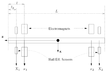
Figure 2: Top view of the MBC500. x₁ (x₃) and x₂ (x₄): horizontal (vertical) displacement from equilibrium measured by the sensors. X₁ (X₃) and X₂ (X₄): horizontal (vertical) displacement of the rotor with respect to the electromagnets.

After this, a linearization of the nonlinear equations is carried out rendering a linear model having x=[x₁ x₂]^T, [x₃ x₄]^T and their time derivatives as state variables. The L/R dynamics of the electromagnets are simplified to i=k_av with i being current and v voltage. A discussion follows, which leads to treat the horizontal and vertical dynamics as decoupled, hence, all experiments were carried out on the design of the horizontal controller. As a consequence, the first model of the horizontal dynamics is the following:

(6)

where y= [y₁ y₂] is the measured voltage output of the horizontal displacement sensors, and u = [u₁ u₂] is the control voltage input of the electromagnets. In order to obtain a validated linear model, an experimental frequency response of the system was obtained. Equation (7) shows the A^o, B^o and C^o matrices which are the matrices that make up the initial model based upon the parameters of Table 1 (see Magnetic Moments LLC 1999; Paden et al., 1996). The latter were used by a nonlinear minimum squares algorithm, as initial conditions for the optimization process leading to final A, B and C matrices which make the model of Eq. (6) fit the experimental frequency response. The A, B and C matrices resulting from the fitting process are shown in Eq. (7) as well.

(7)

A. Flexible Modes

Including a model of the first two bending modes of the rotor proved to be important as far they are likely to receive excitation due to the digital implementation of the designed controllers. The reason for not including any modes higher than the second, is that because of the bandwidth of the actuator's current amplifiers in the electromagnet's L/R circuit, it is practically impossible that these modes would receive excitation. In Morse et al. (1996) a model with four states for the two first bending modes is presented. Here, following the approach of Arredondo et al. (2004), a differential equation with four states is used as well, to model the first two bending modes.

As far as a spectral analysis of the rotor's dynamics is concerned, a clear separation exists between the flexible modes and the rigid body modes. The rigid dynamics show up in the frequency band from DC to about 100 Hz where it rolls-off, and the bending modes are at 777 Hz (first) and 2065 Hz (second). A practical approach for the final model which reflects the rigid and flexible modes, consists in the superposition of three linear blocks as shown in Fig. 3.

Figure 3: Superposition of Rigid and Flexible Dynamics

Let x_fi = be the state of the flexible blocks G_fi in Fig. 3., with i = 1, 2. The form of the state space equations for each of the blocks is as follows:

with

Experimental frequency responses of the system were obtained at the frequency bands of the bending modes. A parameter selection in the A_fi, B_fi and C_fi matrices with i = 1, 2 was carried out seeking an adequate fitting of the experimental frequency responses. The final values of the model parameters for the bending modes are the following:

B. Rotor Eccentricity

Eccentricity is taken into account as external forces acting on the rotor. Rather than a fine identification of the magnitude and direction of the source of the imbalance, a gross estimate of this force is sought. A simplification is carried out in this regard, neglecting the variations in the rotation rate of the shaft. Hence, the eccentric force of the model only depends on the square of the rotation rate. As a consequence, a very simple calculation is carried out for this static case which slightly modifies Eq. (6) in order to take imbalance into account in the rigid dynamics as follows:

(8)

with

where d_o is the diameter of the shaft. The 1/100 factor stems from the assumption that the distance from the true CM to the geometrical axis of the rotor, is in the order of one percent of the shaft's radius (an assumption which is somewhat pessimistic - see Fig. 4.. The ½ factor stems from the fact that two bearings cope with the eccentricity.

Figure 4: Diagram for the eccentricity model

As the G_f1 and G_f2 blocks are concerned, there is a priory knowledge of the frequency band where the ω_im signal appears. This is directly related to the range of rotation rate of the shaft, and it is assumed that this signal does not present and excitation to the bending modes, because of the fact that the maximum rotation rate of the machine is 10000 rpm, i.e. 166 Hz, while the bending modes are in 777 Hz and 2065 Hz.

IV. CONTROL AND SIMULATION RESULTS

In this section the results of the control system design are presented with simulations. The solution of the control problem aims towards the following goals. Stabilize the shaft through a closed loop controller, avoid the excitation of the bending modes (which can actually and eventually be heard in practice) and render adequate imbalance rejection in a range of rotating rates as broad as possible.

In order to evaluate performance of the designed controllers, frequency responses of the Output Sensitivity functions will be presented. In this problem, good tracking is not the main goal, especially since it would demand a high loop gain in low frequency, which in turn would lead to a peak in the sensitivity function at a frequency close to the cross-over frequency. This is because of fundamental limitations of closed loop systems in presence of unstable poles (see Morse Thibeault and Smith, 2002; Seron et al., 1997). Another way to evaluate performance will be through simulated time responses to step inputs, which should show no excitation of the bending modes and acceptable transient behavior. In particular these responses will be compared with the transient behavior of an controller. Finally, in the following section, experimental results are shown. The spinning of the shaft will be the ultimate test. Time responses to the equivalent sinusoidal inputs will be observed in the simulations of this section as well.

A. LPV design

Together with the LPV design, an controller is obtained with the intention of comparing it with the LPV. The statement of the problem is the same for both. The details of the LPV approach are presented first, with remarks concerning the feasible parameter variation set. Regarding the Robust methodology, the controller aims towards the operation of the rotating machine with a fixed rotating rate of 5000 rpm. The result gives a reference of the desirable γ performance factor for the LPV design and this in turn, is related to the subject of the size of the parameter variation set.

Anticipating the final remarks, an immediate conclusion of this work is that the feasible parameter variation set for the LPV problem is not satisfactory for this application. Even though a natural parameter variation set exists (_n = 0-10000 rpm), which is given by the manufacturer of the Magnetic Bearing Experiment, it was not possible with this range to obtain a feasible solution to the γ-performance LPV control problem with pole placement constraints (Sect. II).

Different parameter variation sets were tried in order to establish in what cases a solution to the control problem existed, and how performance was affected by the size of the parameter variation set (given feasibility). Before turning to the details of this trial and error process, the statement of the control problem, i.e. the augmented plant with the weighting functions, will be presented.

The diagram of Fig. 5 shows the blocks involved in the augmented plant. In order to simplify the problem statement and with the objective of keeping the parameter varying part of the problem circumscribed to the W₁ block, a minor modification is carried out on Eq. (8). As a result, the r² factor multiplying the k_im constant is moved into the W₁ weight and the G_r transfer matrix is as follows:

(9)

with

It is remarked that the r² factor that accounts for the increase in the magnitude of the imbalance force (as the rotation rate grows), has been removed from Eq. (8) to obtain the description of the G_r(s) transfer matrix. As the and LPV methods used for synthesis in this application consider all disturbance inputs to be signals in ₂ (i.e. d₁, d_{2 2}), we resorted to including the W₁ block, a variable gain, variable frequency bandpass prefilter, that accounts for the fact the true ω_im signal (see Eq. (8)) is a sinusoidal signal of known frequency whose amplitude depends on r². As it was previously mentioned, this disturbance signal serves the purpose of modelling the imbalance forces acting on the rotor. As a sinusoidal signal, its frequency is given by the rotation rate of the shaft. Given a fixed rotation rate r, the transfer function of the W₁ filter turns out to be as follows:

(10)

Notice that the state space representation of Eq. (10) shows the affine dependence of the state space matrices of the filter on r and r². When setting up the LPV synthesis problem, the existing relation between r and r² will be neglected. As far as the synthesis method concerns, the ω ₁ weighting function depends affinely on two independent parameters p₁=r and p₂=r². No advantage is taken from knowing that p₂ = p₁² and in that way, the approach is slightly conservative.

Figure 5: Augmented Plant

On the other hand, the W_u(s) and W_Δ(s) filters are shaped in frequency with the following objectives in mind. In the case of W_u(s), penalize any control action above a given ω_u frequency and in the case of W_Δ(s), give the synthesis algorithm the frequency information concerning the bending modes. The transfer functions of the weights are as follows:

with

W_Δ(s) can be thought of as a weighting function for a family of plants with additive uncertainty and W_u(s) is the weighting function penalizing control action in high frequency. Additive uncertainty is taken into account, as the norm reduction of the mapping from d₂ to y_Δ (see Fig. 5) is addressed by the synthesis algorithm minimizing the norm of the mixed sensitivities operator mapping to .

TheW₂(s) weighting transfer function for the controlled output is as follows:

with for ω_l = 2π60rad/s for k_l = 2.

The shape of the ω₂ and ω_u filters follows typical guidelines for the choice of closed loop bandwidth and control bandwidth. Avoiding a high peak in the magnitude of the frequency response of the sensitivity transfer function is sought as well (see Zhou, 1998; and Zhou, 1996). An iterative process was carried out as well for the final fine tuning of these values.

Parameter Variation Set

The general observation concerning the parameter variation set is that given a maximum value for the rotation rate r_max, the reasonable parameter variation set for the two parameter (r, r²) LPV system is

with r_min = 0.8 r_max. This rule was empirically established following the aforementioned criteria of feasibility of the corresponding LMI problem and performance index within three times the performance index of the Robust problem resulting from holding the parameter rfixed at r = r_max.

Table 2 shows the and LPV control designs that were attempted. Because of the infeasibility of the optimization problem for the whole [0, 10000] rpm range, the [4000, 5000] rpm range was tried in order to draw conclusions. The design carried out, corresponds to r = 5000 rpm. As can be seen in the table, a greater interval was infeasible.

Table 2: Performance Index and Parameter Variation Set

B. Frequency Responses and Simulation Results

In the present section frequency response graphics are shown, as well as simulated time responses.

Notice in Fig. 6 that the design, specifically designed for a fixed rotation rate, renders a reduction of the sensitivity at the expected rotation rate frequency. On the other hand the frequency responses of the LPV controller calculated for r=r_max and r=r_min, show higher gains at low frequency than the .

Figure 6: Frequency response of the maximum singular value the Output Sensitivity Transfer Functions. Solid line: H_∞, dash-dot line: LPV(r_max), dots line: LPV(r_min).

Figure 7 shows time responses to step inputs to be followed by the x₁ output. Recall that good tracking is not a must, but it cannot be too poor either. If that were the case, the system might fail to stabilize the rotor for r=0 rpm.

Figure 7: Step Responses. Solid line: , dash-dot line: LPV(r_max), dots line :LPV(r_min).

Figures 8 and 9 show time responses to sinusoidal inputs injected on both sides that simulate imbalance forces.

Figure 8: Responses to Sinusoidal Force of frequency r=r_max=5000 rpm. Solid line: dash-dot line: LPV(r_max).

Figure 9: Responses to Sinusoidal Force of frequency r=r_min=4000 rpm. Solid line: dots line: LPV(r_min).

These are to be rejected. Notice that the design performs better than the rest at the specific frequency it was designed for (r_max = 5000 rpm) while achieving a decent result for the low rotation rate the LPV was designed for (r_max = 4000 and 8000 rpm). Naturally, the LPV performs better than the in this case, but not by far.

V. EXPERIMENTAL RESULTS

In this section, the experimental results are presented. With respect to the experimental results presented in Ghersin et al. (2007), the difference resides in the successful implementation of an LPV controller. It must be said that the synthesis with pole placement constraints for this case, rendered an unstable controller. As a consequence, the Robust controller was redesigned without pole placement constraints as in Ghersin et al. (2007) but with the modifications on the augmented plant introduced here. The results obtained are similar while the controller remains suitable for implementation. The LMI region used for the LPV synthesis with pole placement constraints of this paper was the following:

In terms of the α and β matrices of Eq. (1), this region gives scalars α = -2π 2100 and β= -1. In spite of the fact that this is a very simple LMI region as the size of α and β is concerned, the computation time of the LPV controller is considerably increased.

Figures 10 to 14 show the responses of the experimental equipment for three different controllers with the machine operating at 4000 and 5000 rpm respectively. The measured signals, displayed in an oscilloscope in XY mode, are the horizontal (x₁) and vertical (x₃) displacements of the rotor on the left hand side of the machine. The displayed voltage signals correspond with displacement with a factor of 1 mm per volt (i.e. 100 mV is 0.1 mm). The scale of the horizontal and vertical axes for all Figs. is 200 mV/div. Notice that only the excursion in the X axis matters in order to evaluate the performance of the designed controllers. The control of the vertical axes x3 and x4 was left to the internal compensator. Figures 10 and 11 show the responses with the internal compensator of the MBC500, Fig. 12 with the Robust controller designed for imbalance forces at 5000 rpm (in the sequel ⁵⁰⁰⁰) and Figs. 13 and 14 with the LPV controller. The response of the ⁵⁰⁰⁰(Fig. 12) shows the filtering of imbalance forces that the controller does at 5000 rpm which is remarkable. As it stems from Figs. 13 and 14 the remarkable aspect of the performance of the LPV controller is that it greatly improves the performance with respect to the internal compensator especially for the 4000 rpm rate (67 Hz) a

Figure 10: Experimental Responses to 4000 rpm. x and y axes: Internal Compensator.

Figure 11: Experimental Responses to 5000 rpm. x and y axes: Internal Compensator.

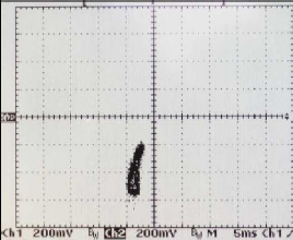
Figure 12: Experimental Responses to 5000 rpm. x-axis controller: ⁵⁰⁰⁰ , y-axis controller: Internal.

Figure 13: Experimental Responses to 4000 rpm. x-axis controller: LPV, y-axis controller: Internal.

Figure 14: Experimental Responses to 5000 rpm. x-axis controller: LPV, y-axis controller: Internal.

frequency within the open loop bandwith. The performance of the ⁵⁰⁰⁰controller at 4000 rpm wass between the LPV and the internal compensator.

VI. CONCLUDING REMARKS

The use of LPV synthesis methods for this application is a priory appealing, motivated by references such as Matsumura et al. (1996) where traditional gain scheduling is used, and by the results obtained for this work both experimental and simulated. In spite of the benefits it provides in terms of smooth scheduling and guaranteed stability, the method has shown its problems as far as the parameter range is concerned. This issue suggests the use of less conservative techniques such as LPV synthesis based upon Parameter Dependent Lyapunov Functions (Wu et al., 1996; see also Apkarian and Adams, 1998). The use of more advanced LFT techniques, which give less conservative solutions, such as Scherer (2001) is another possible direction for LPV re-design. Regarding the techniques of Scherer (2001), preliminary research of the authors on the subject, has shown their practical implementation is yet not a fully solved problem (see Trangbæk, 2001; Ghersin, 2006).

The matter of fast dynamics that prevents the easy implementation and simulation of controllers has been addressed through the technique of section II, which is pretty simple as the complexity in its application is not greater than that of control. This technique even renders an LMI problem with a finite number of constraints (at the expense of being conservative, perhaps). The results presented in Ghersin et al. (2007) obtained with this technique were not useful (the LPV controller was unstable), while the difference with this successfully implemented controller was a matter of fine tuning. This can be understood considering that neither LPV control with pole placement constraints nor control with pole placement constraints guarantee stable controllers.

---

¹ Linear Matrix Inequality.
² Semidefinite Programming.

ACKNOWLEDGMENTS
The research reported in this work was partially supported by the following institutions: Agencia Nacional de Promoción Científica y Tecnológica of Argentina through grants PICT 97' BID OC/AR 1758 and PICT 99' BID OC/AR 7263, the Universidad de Buenos Aires (UBA) through grant PC 98'-00' TI34 and the Universidad Nacional de Quilmes (UNQ) through grant PUNQ 0530/07. The experimental work of this research was carried out at the Space Access Program Lab at the National Commission of Space Activities of Argentina (CONAE).

REFERENCES
1. Apkarian, P., "On the discretization of LMI synthesized linear parameter-varying controllers," Automatica, 4, 655-661 (1997).         [ Links ]
2. Apkarian, P. and R.J. Adams, "Advanced gain-scheduled techniques for uncertain systems," IEEE Transactions on Control Systems Technology, 6, 21-32 (1998).         [ Links ]
3. Arredondo, I., J. Jugo and V. Etxebarria, "Modelización y control de un eje sustentado mediante levitación magnética activa," Proceedings of the XXV Jornadas de Automática, CEA-IFAC (2004).         [ Links ]
4. Becker, G.S. and A. Packard, "Robust performance of LPV systems using parametrically-dependent linear feedback," Systems and Control Letters, 23, 205-215 (1994).         [ Links ]
5. Chilali, M. and P. Gahinet, "H_∞ control design with pole placement constraints: An LMI approach," IEEE Transactions on Automatic Control, 41, 358-367 (1996).         [ Links ]
6. Ghersin, A.S., "Applicability of LPV synthesis with full block multipliers," Proceedings of the XX Congreso Argentino de Control Automático - AADECA 2006, Buenos Aires - Argentina (2006).         [ Links ]
7. Ghersin, A.S., R.S. Smith and R.S. Sánchez Peña, Identification and Control: the Gap between Theory and Practice, Springer (2007).         [ Links ]
8. Ghersin, A.S. and R.S. Sánchez Peña, "LPV control of a 6 DOF vehicle," IEEE Transactions on Control Systems Technology, 10, 883-887, (2002).         [ Links ]
9. Magnetic Moments, LLC, MBC500 Manual (1999).         [ Links ]
10. Matsumura, F., T. Namerikawa, K. Hagiwara and M. Fujita, "Application of gain scheduled H_∞ robust controllers to a magnetic bearing," IEEE Transactions on Control Systems Technology, 4, 484-493 (1996).         [ Links ]
11. Morse, N., R. Smith and B. Paden, Magnetic bearing lab #1: Analytical modeling of a magnetic bearing system (1996).         [ Links ]
12. Morse Thibeault, N. and R.S. Smith, "Magnetic bearing measurement configurations and associated robustness and performance limitations," ASME Journal of Dynamic Systems, Measurement and Control, 124, 589-598 (2002).         [ Links ]
13. Paden, B., N. Morse and R. Smith R., "Magnetic bearing experiment for integrated teaching and research laboratories," Proceedings IEEE Conference on Control Applications (1996).         [ Links ]
14. Scherer, C.W., "LPV control and full block multipliers," Automatica, 37, 361-375 (2001).         [ Links ]
15. Seron, M.M., J.H. Braslavsky and G.C. Goodwin, Fundamental Limitations in Filtering and Control, Springer-Verlag, London (1997).         [ Links ]
16. Trangbæk K., "Linear parameter varying control of induction motors," PhD Thesis Aalborg University (2001).         [ Links ]
17. Wu, F., X.H. Yang, A. Packard and G.S. Becker, "Induced L2-norm control for LPV systems with bounded parameter variation rates," International Journal of Nonlinear and Robust Control,6, 2379-2383(1996).         [ Links ]
18. Zhou, K., Robust and Optimal Control, Prentice-Hall (1996).         [ Links ]
19. Zhou, K., Essentials of Robust Control, Prentice-Hall (1998).         [ Links ]

Received: March 30, 2009.
Accepted: October 12, 2009.
Recommended by Subject Editor: José Guivant.