Interactive remeshing for navigation over landscape models

M. V. Cifuentes^†, M. J. Venere^‡ and A. Clausse^‡

^† CICPBA - Universidad Nacional del Centro, 7000 Tandil, Argentina
^‡ CNEA- Universidad Nacional del Centro, 7000 Tandil, Argentina
{cifuente, venerem, clausse}@exa.unicen.edu.ar

Abstract — The performance of an algorithmic procedure to visualize digital landscapes based in the dynamic control of the size of the model is presented. Approximate representations are produced taking into account criteria relative to the observer position and the local curvature of the terrain. The algorithm leads to substantial reductions of the size of the final meshes, lowering the rendering costs down to 5%. An application of the algorithm is tested on a model of the Colorado Canyon is shown.

Keywords — Surface Simplification. Landscape Visualization. Computational Geometry. Polygonal Mesh.

---

I. INTRODUCTION

Virtual reality applications based on outdoor scenarios demand realistic and efficient topographic representations. The current trend is to abandon models based on special effects such as projected images or synthetic representations, resorting instead to real digital elevation models (DEMs). Basically a DEM is a grid where each cell is associated with a pair of geo-referenced coordinates (e.g. geodesic or Gauss Kruger) and a corresponding terrain height, leading to a digital representation of a fraction of the earth surface within a given resolution. Current DEMs use tens and even hundreds of millions of cells. Such a huge volume of data is necessary in many applications, but it is hard to visualize interactively, particularly if interactive navigation is involved (Duchaineau et al., 1997; Gobbetti et al., 2006 and Livny et al., 2007). The mesh data often exceed the available memory, and this problem is more dramatic if texture maps are involved (Döllner et al., 2000).

In the last decades several efficient algorithms and techniques were developed to digitally represent terrains preserving the quality of the visualizations while keeping fast access to the data. One of the most interesting strategies is mesh simplification by recursive decomposition. In particular, the adaptive simplification algorithms start from the simplest version of the original model and subsequently add greater detail enhancing the quality of the primal model (Balmelli et al., 1998; Hoppe, 1998; Pajarola, 1998; Röttger et al., 1998; Lindstrom and Pascucci, 2002; Pajarola et al., 2002 and Pajarola and Gobbetti, 2007). DeHaemer and Zyda (1991) have successfully applied this technique in DEMs with an algorithm that preserves the topology.

In this article, a variant of the adaptive simplification methods is presented and applied to DEMs visualization. A hierarchy quadtree with restrictions and templates associated to the end nodes is used to generate the final surface ensuring conformal triangulation and avoiding major changes in the size of the mesh polygons. The basic guiding criterion to the coarsening process is the local curvature of the represented surface (Cifuentes et al., 2004). Subsequent enhancement is achieved by introducing a refinement according to the position of the observer (Gerstner, 1999). The result is a dynamic mesh that is extracted from the quadtree hierarchy which mutates following the movement of the observer. The size of the problem can be reduced one order of magnitude; and even more if some quality loss is accepted.

II. COARSENING GUIDED BY CURVATURE

Let us start with a DEM supported by a regular mesh of squared pixels. The height of the terrain, h_ij, is provided for every Δ×Δ cell located in each vertex (i,j). One reasonable criterion to simplify this model is to decrease the number of pixels in regions where the curvature is small (Miao et al., 2009). The underlying principle is that in order to obtain similar visualization qualities smoother regions can be represented by fewer cells than rougher regions.

To construct a simple local curvature indicator, we propose to use the Frobenius norm of the curvature tensor in each vertex, given by:

	, (1)

where Gx_ij and Gy_ij are the gradient components in each direction and can be efficiently approximated by

	, (2)
	, (3)

Accordingly, the cumulative curvature of a given set S of neighbour vertices is defined as

(4)

Then, the procedure to simplify the mesh is as follows:

1. Let the entire domain N × M be the root of a tree.
2. Divide each branch of the tree in four subsets cutting through the apothems.
3. Calculate the cumulative curvature, K, of each subset according to Eq. 4.
4. Continue applying this procedure to every subset until the cumulative curvature of all the branches are below certain predefined upper bound, K_max.

A hierarchy of meshes of different complexity is generated through the subsequent divisions leading to a quadtree representation whose k-level nodes are squares with side-length L / 2^k, being L size of the original domain. The smallest nodes are called leaves. According to the quadtree structure, the cumulative curvature of each k-level square is calculated before adding the corresponding cumulative curvature of its four descendents. Figure 1 shows the final structure obtained with the mentioned procedure for a simple case of a surface with a change in the slope.

Fig. 1: Example of quadtree decomposition.

The applied data structure provides a simple and fast way to localize any node, organizing each quadtree level in an array. The ancestor of a k-level node localized at (i,j) is a (k-1)-level node localized at (i/2, j/2), the descendants are (k+1)-level nodes localized at (2i, 2j), (2i+1, 2j), (2i, 2j+1) and (2i+1, 2j+1). This design improves the performance of the algorithm because it quickly builds a restricted quadtree and the corresponding polygonal mesh of the surface.

A. Conformed mesh

As in any other multigrain representation, the proposed solution should be complemented by a conformation correction in order to avoid holes in the mesh wherever two different coarsening levels touch each other. For that purpose, every adjacent region should not differ in more than a single coarsening level. The simplest solution is to close the surface discontinuities with additional polygons; however many of these new elements will have anomalous aspect ratios (Von Herzen and Barr, 1987). In our case, we adopt an alternative technique that yields better visualizations (Rivara and Vénere, 1996). The final mesh is conformed using four types of triangles having good aspect ratios. The number of additional triangles required is O(NumTerminals^1/2).

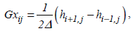
Surface continuity at junctions separating regions differing in a single coarsening level are obtained by realizing that there are just 16 possible situations, which are shown in Fig. 2. To resolve the discontinuities, the template solution should be applied to the correspondent situation. Figure 3 shows the final result

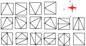
Fig. 2: Templates used for triangulate the terminal nodes. Red points are problematic vertex causing holes in the mesh.

Fig. 3: Mesh before and after applying templates.

III. REFINEMENT GUIDED BY THE DISTANCE TO THE OBSERVER

Lindstrom and Pascucci (2002) and Gerstner (2003) propose to use the distance to the observer as a criterion to deal with fast landscape navigations. The underlying principle is that regions farther from the observer require fewer details than closer ones. Hence, to simulate navigations the coarsening should change following the observer movement. Following this concept, we propose the following dynamic criterion to integrate the targets of curvature and distance to the observer:

(6)

where d is the distance from the observer to the centre of the region expressed as a fraction of the main diagonal of the total domain, ω is a control parameter representing the relative importance of the observer distance respect to the curvature, and K'_max is a tolerance value imposed by the user. The parameter ω controls the visual appearance of the representation. Thus, when , the curvature dominates the coarsening process, whereas as ω increases an additional refining is imposed in regions closer to the observer. Figure 4 shows the effect of the distance to an observer for the case shown in Fig. 1, using ω = 70 and K_max = 0.001.

Fig. 4: Remeshing according to local curvature (left) and observer's location (right). The visualization parameters of Eq. 6 are ω = 70 and K_max = 0.001.

A breath-first algorithm was implemented starting with the construction of a passive base coarsening in a quadtree generated with the curvature indicator alone (i.e., ω=0). The dual curvature-distance indicator (ω>0) was then applied to generate active coarsening, which is dynamically constructed during navigations using the passive coarsening as primitive. To generate an active hierarchy, the search begins at the root node of the passive tree, and proceeds towards the leaves activating and deactivating nodes according to the criterion given by Eq. 1. Simultaneously, the mesh is conformed properly in order to avoid discontinuities. Figure 5 shows the passive hierarchy (i.e., the whole tree) and the active hierarchy (dashed regions). The terminal nodes (red) constitute the final triangulation.

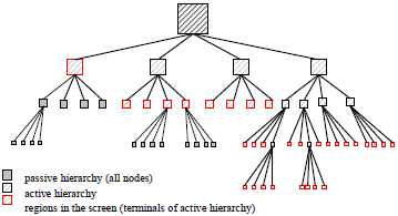
Fig. 5: Active and passive hierarchies.

IV. RESULTS

The remeshing algorithm was tested on a synthetic DEM and in two real landscapes: the Colorado Canyon and the Lake Nahuel-Huapi. The synthetic model consists of a regular square grid, representing an ideal slope flattened at the top and the bottom. The number of triangles of the original mesh is 131,072.

Table 1 shows the performance of the remeshing guided by curvature (ω=0). It can be seen that in this ideal case there is a substantial reduction on the number of triangles, even when the tolerance is null (i.e., only the strictly planar regions are reduced). As expected, the number of forced divisions to eliminate discontinuities decreases as the tolerance increases. Figure 6 shows the variation of the number of triangles of the final mesh with the curvature tolerance.

Table I: Performance of the remeshing according to curvature. The input model is the regular square mesh of 131,072 triangles shown in Fig. 6.

Fig. 6: Relation between the number of triangles and the tolerance.

Figure 7 shows visualizations of the synthetic terrain for different tolerances. Due to the simplicity of the model, even a crude coarsening represents quite well the original surface. It can be seen that the algorithm forces a denser meshing at the bands where the curvature is higher. The error introduced by the coarsening can be quantified by calculating the volume enclosed between the actual model and the remeshing. It can be seen in Fig. 8 that the error is higher as the curvature tolerance increases, following the law

Fig. 7: Original mesh of 131,072 triangles (a) and data approximations of 10,224 triangles (b), 1,072 triangles (c) and 32 triangles (d).

Fig. 8: Effect of the curvature tolerance on the representation error.

Figure 9 shows the remeshing resulting from three different positions of the observer keeping constant the parameter ω =70. It can be seen that the density of triangles increases in the regions closer to the observer (blue point), prioritizing the rendering around him, as happens in visualizations of real landscapes.

Fig. 9: Interactive remeshing during navigation.

Note that although the resulting approximation is constructed with about 1% of the polygons of the original DEM, the observer neighbourhood maintain the same density as the mesh generated with K_max = 0.001.

Fig. 10 shows a dynamic mesh representation of the Colorado Canyon, starting from a 16 million triangles DEM. The passive mesh (ω = 0) has about 20 thousand triangles. Running on a 3 GHz 1Gb-RAM Pentium IV and GeForce FX 5200, the passive mesh is generated in 0.28 s, each remeshing takes 12 ms and the rendering 29 ms. Following a remeshing strategy that actualize the active hierarchy only when the region closest to the observer violates the tolerance criterion, rendering rates of 20 f/s can be achieved.

Fig. 10: Remeshing of Colorado Canyon MDE (ω = 15). Observer is located at red point.

Figure 11 shows visualizations of the landscape of Lake Nahuel Huapi in southern Patagonia. The left figures are the remeshing used to represent the corresponding pictures on the right. Note that as the observer get close to a region the corresponding geometry is enriched in details due to the increasing local triangle density.

Fig. 11: Views of the navigation with interactive remeshing of the model (DEM of Lake Nahuel Huapi, Argentina).

Figure 12 shows the sensitivity of the remeshing density with the parameter ω. It can be seen that the number of triangles is greatly reduced as ω increases. Figure 13 shows the visualization error, calculated as the volume enclosed between representations, goes as , with x decreasing slightly with ω (x = 1.6 forω = 5, x = 1.5 for ω = 15).

Fig. 12: Influence of the parameter ω on the remeshing density.

Fig. 13: Effect of the tolerance on the error of the dynamic representation.

V. CONCLUSIONS

An algorithm to dynamically reduce the number of triangles required to visualize digital elevation models during navigations was proposed and tested. The algorithm takes into account the curvature of the terrain and the distance to the observer, leading to substantial reductions of the complexity of the final meshes, lowering the rendering cost down to 5% in the worst case scenario studied. The strategy of an active hierarchy supported by a passive hierarchy showed good performances, especially when the observer navigates through under-detailed regions. The memory saving of the technique is also quite powerful, reaching in all cases a 90% reduction of memory space, while keeping the visual appearance of the model.

REFERENCES
1. Balmelli, L., S. Ayer and M. Vetterli, "Efficient Algorithms for Embedded Rendering of Terrain Models," Proceedings IEEE International Conference on Image Processing, 914-918 (1998).         [ Links ]
2. Cifuentes, M.V., M. Vénere and A. Clausse, "Un algoritmo para la simplificación de modelos digitales de elevación," 33º Jornadas Argentinas de Informática e Investigación Operativa (2004).         [ Links ]
3. DeHaemer, M. and M. Zyda, "Simplification of objects rendered by Polygonal Approximations," Computers & Graphics, 15, 175-184 (1991).         [ Links ]
4. Döllner, J., K. Baumann and K. Hinrichs, "Texturing techniques for terrain visualization," IEEE Computer Society Technical Committee on Computer Graphics, 227-234 (2000).         [ Links ]
5. Duchaineau, M., M. Wolinsky, D. Sigeti, M. Miller, C. Aldrich and M. Mineev-Weinstein, "ROAMing terrain: real-time optimally adapting meshes," Proceedings of the 8th conference on Visualization, 81-88 (1997)         [ Links ]
6. Gerstner, T., Multiresolution Compression and Visualization of Global Topographic Data, Technical report, Institut für Angewandte Mathematik, Universität Bonn (1999).         [ Links ]
7. Gerstner, T., Top-Down View-Dependent Terrain Triangulation using the Octagon Metric, Technical report, Institute of Applied Mathematics, University of Bonn (2003).         [ Links ]
8. Gobbetti, E., F. Marton, P. Cignoni, M.D. Benedetto and F. Ganovelli, "C-BDAM - Compressed Batched Dynamic Adaptive Meshes for Terrain Rendering," Computer Graphics Forum, 25, 333-342 (2006).         [ Links ]
9. Hoppe, H., "Smooth View-Dependent Level-of-Detail Control and its Application to Terrain Rendering," Proceedings IEEE Visualization, 98, 35-42 (1998).         [ Links ]
10. Lindstrom, P. and V. Pascucci, "Terrain simplification simplified: A general framework for view-dependent out-of-core visualization," IEEE Transaction on Visualization and Computer Graphics, 8, 239-254 (2002).         [ Links ]
11. Livny, Y., Z. Kogan and J. El-Sana, "Seamless patches for GPU-based terrain rendering," Proceedings of WSCG 2007, 201-208 (2007).         [ Links ]
12. Miao, Y., R. Pajarola and J. Feng, "Curvature-aware Adaptive Re-sampling for Point-Sampled Geometry," Computer Aided Design, 41, 395-403 (2009).         [ Links ]
13. Pajarola, R., "Large scale Terrain Visualization using the Restricted Quadtree Triangulation," Proceedings IEEE Visualization, 19-26 (1998).         [ Links ]
14. Pajarola, R., M. Antonijuan and R. Lario, "QuadTIN: Quadtree based Triangulated Irregular Networks," Proceedings IEEE Visualization, 395-402 (2002).         [ Links ]
15. Pajarola, R. and E. Gobbetti, "Survey of semi-regular multiresolution models for interactive terrain rendering," The Visual Computer, 23, 583-605 (2007).         [ Links ]
16. Rivara, C. and M. Vénere, "Cost Analysis of the longest-side refinement algorithm for triangulations," Engineering with Computers, 12, 224-234 (1996).         [ Links ]
17. Röttger S., W. Heidrich, P. Slusallek and H.P. Seidel, "Real-Time Generation of Continuous Levels of Detail for Height Fields," Proceedings of WSCG, 315-322 (1998).         [ Links ]
18. Von Herzen, B. and A.H. Barr, "Accurate triangulations of deformed, intersecting surfaces," Proceedings ACM SIGGRAPH, ACM Journal Computer Graphics, 4, 103-110 (1987).         [ Links ]

Received: December 15, 2008.
Accepted: October 12, 2009.
Recommended by Subject Editor: José Guivant.