


Services on Demand
Journal

Article
 English (pdf)
 Article in xml format
 Article references
 Send this article by e-mail
Indicators
-
 Cited by SciELO
Related links
-
 Similars in
SciELO
Similars in
SciELO
Share

 Permalink
Latin American applied research
Print version ISSN 0327-0793
Lat. Am. appl. res. vol.41 no.2 Bahía Blanca Apr. 2011
ARTICLES
A comparison of metaheuristics algorithms for combinatorial optimization problems. Application to phase balancing in electric distribution systems
G.A. Schweickardt†, V. Miranda‡ and G. Wiman*
† Instituto de Economía Energética/CONICET - Fundación Bariloche - Av. Bustillo km 9,500 - Centro Atómico Bariloche - Pabellón 7, Argentina. gustavoschweickardt@conicet.gov.ar
‡ INESC Porto - Instituto de Engenharia de Sistemas e Computadores do Porto and FEUP - Fac. Engenharia Univ. Porto P. República 93 - 4050 Porto, Portugal. vmiranda@inescporto.pt
* Universidad Tecnológica Nacional - FR BA, Ext. Bariloche - Fanny T. de Newbery 111, Bariloche, Argentina gwiman@utn.frba.edu.ar
Abstract — Metaheuristics Algorithms are widely recognized as one of most practical approaches for Combinatorial Optimization Problems. This paper presents a comparison between two metaheuristics to solve a problem of Phase Balancing in Low Voltage Electric Distribution Systems. Among the most representative mono-objective metaheuristics, was selected Simulated Annealing, to compare with a different metaheuristic approach: Evolutionary Particle Swarm Optimization. In this work, both of them are extended to fuzzy domain to modeling a multi-objective optimization, by mean of a fuzzy fitness function. A simulation on a real system is presented, and advantages of Swarm approach are evidenced.
Keywords — Metaheuristic Algorithm; Swarm Intelligence; Fuzzy Sets; Electric Distribution; Phase Balancing.
I. INTRODUCTION
Metaheuristics Algorithms are widely recognized as one of more practical and successful approaches to solve combinatorial problems. However, the original formulations have been oriented to mono-objective optimizations. Many proposal of extensions to multi-objective domain have been established, but each formulation has showed particular advantages and limitations, in general, over certain kind of problems. Does not exist the "best multiobjective metaheuristic algorithm", but some algorithms are more appropriates for certain problems. Such is the case of Phase Balancing in Low Voltage Electric Distribution Systems (LVEDS), when a classic programming approach is not addressed to solve it. The balance is referred to the loads in the feeders of a LV network in an EDS. The classic approach, has demonstrated major limitations, as it will be discussed. For this reason, a metaheuristic approach is an alternative that may produce very good results.
This work is organized as follows: in the section II.A the problem of Phase Balancing is presented. It describe the no desired effects that produce an elevate unbalance degree in the loads of a low voltage (LV) feeder. In section II.B are described the principles of two mentioned metaheuristics: Simulated annealing (SA) and Evolutionary Particle Swarm Optimization (EPSO). In section II.C, an introduction of the static fuzzy decision is presented, and the extension of the SA and EPSO algorithms to fuzzy domain, by mean of a fuzzy fitness function, is proposed for solve multi-objective optimizations. Two models, designed as FSA and FEPSO, specialized to solve the Phase Balancing Multi-objective Problem, are obtained. Lastly, in the section II.D, a simulation on a real LV feeders system is presented and the results, obtained from FSA and FEPSO, are compared. The conclusions are presented in the section III.
II. METHODS
A. The Problem of Phase Balancing
The most LV networks of an EDS are three-phase systems, physically defined by feeders with three conductors, one per phase (feeders system). If all loads of each conductor-phase were three-phase (with the same value in each phase) then the system would be balanced. However, feeders loads in a LV network, for low incomes residential areas, are commonly single-phase. Original feeders system design, depends on accuracy of the given load data and, even maximizing this accuracy, there will always be certain unbalance degree, due to single-phase loads. A high unbalance degree, produces high voltage drops, high power and energy losses and low reliability. For this reason, such degree must be as low as possible. For the purpose of this paper, LV feeders system will have only single-phase loads. A formulation to the general problem of Phase Balancing, in this context, can be expressed as follows:
Min { LossT ; I(Δu) ; |I[o]|f } (1)
Subject to:
|I[R]|f ≤ IMax (2)
|I[S]|f ≤ IMax (3)
|I[T]|f ≤ IMax (4)
where the subindex f, refers to the output of substation connected to the principal feeder of the system; LossT are the total active power loss of system and I(Δu) is an index that depends on voltage drops.
I[o]f (homopolar component) satisfy the equation:
I[R]f+I[S]f +I[T]f = 3 x I[o]f (5)
If the system is balanced, then |I[o]|f = 0.
The sub index [R], [S] and [T], refers to each phase of system. In addition, three constraints are imposed: the intensities in each phase at the output, must be less than the phase line capacity, IMax, Eq. (2), (3) and (4). The problem can be seen as a set of swapping single phase loads or a load assignment to lines. For example, a single phase load can only be assigned to either phase [R], [S] or [T] (see Fig. 1). This assignment should be executed until the objectives (1) are satisfied.

Figure 1 - Single Phase loads and Balance by Phase Swapping in some loads
In the Fig. 1, the line-dotted rectangles represent nodes in which groups of single phase loads are connected (i.e. residential customers). Swaping the phases (double-arrow curves), the objectives functions (1) are evaluated by mean of a three-phase load flow. Pi is the active power and Qi is a reactive power connected at the node i. Phase Balancing has several significant benefits, such as improving power quality and reliability, and the utilization factor. More details are presented in the section II.D.
This problem is clearly combinatorial: if there are 3 phases and n loads that can be swapping, then the number of states of search space for the solution, is 3n. In the reference (Zhu et al., 1998) is proposed to solve it a model based in Linear Mixed-Integer Programming, but it exhibit significant limitations, such as: a) the problem is not linear, and the linear formulation is valid if the current of each individual load is constant. This situation does not occurs in practice; b) the model requires a convex set of parameters, of summatory 1, as subjective weights for each node to weigh the importance of its unbalance degrees. This simple formulation to Multi-Objective Linear Optimization, is a poor approach to search a global minimum in the objectives functions (1).
A metaheuristic approach, perform a better search in the solutions space, because it not require to know, essentially, the characteristic of each objective function.
B. The Metaheuristics SA and EPSO
B.1. Simulated Annealing (SA)
The concept of Simulated Annealing in combinatorial optimization was introduced by Kirkpatrick et al. (1983). SA appears like a flexible metaheuristic that is an adequate tool to solve a great number of combinatorial optimization problems. It is motivated by an analogy to annealing in solids and the idea comes from a paper published by Metropolis et al. (1953). The Metropolis algorithm simulated the cooling of material in a heat bath. This is the process know as annealing. It consists on two steps: a) the temperature is raised to a state of maximum energy and b) the temperature is slowly lowered until a minimum energy state, equivalent to thermal equilibrium, is reached. The structural properties of the system, depends on the rate of cooling. If it is cooled slowly enough, large crystals will be formed. However, if the system is cooled quickly, the crystals will contain imperfections. Metropolis's algorithm simulated the material as a system of particles.
In order to more clearly explain the SA metaheuristic, is possible present an analogy between a physical system, with a large number of particles, and a combinatorial problem. This analogy can be stated as follows:
- The solutions of combinatorial problem are equivalent to the physical system states;
- The attributes of solutions are equivalent to the energy of different states;
- The control parameter in the combinatorial problem is equivalent to the temperature of physical system.
The evolution of the solution algorithm is simulated using probabilistic sampling techniques, supported by successive generation of states. This process begins with an initial state, i, evaluated by an energy function, E(i). After generating and analyzing a second state, j, E(j), it is performed an acceptation test. The acceptance of this new solution, j, depends on a probability computed by:
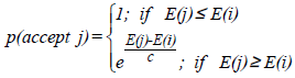 | (6) |
where c is a positive real number, c = kB x T; kB is a constant (called Bolzman constant, in Metropolis's Algorithm) and T is a temperature of system.
A procedure is defined, in pseudo-code, as follows:
Minimize f(i) for i ∈ S → Search Space
Begin Procedure SA
1. set starting point i = i0
2. set starting temperature T = T0 and cooling rate: 0 < a < 1;
3. set NT (number of trials per temperature);
4. while stopping condition is not satisfied do
5. for k ← 1 to NT do
6. generate trial point j from Si using q(i, j);
7. accept j with probabylity p(accept j) (eq. 6);
8. end for
9. reduce temperature by T ← T x a;
10. end while
End Procedure SA
Si is a Neighborhood of solution i: is a set of discrete points j satisfying j ∈ Si ⇔ i ∈ Sj. The generation function of Si is q(i, j) defined externally.
B.2. Evolutionary Particle Swarm Optimization (EPSO)
The metaheuristic EPSO, is built over the concepts of Evolution Strategies (ES) and Swarm Intelligence (SI). Under the name of Evolution Strategies and Evolutionary Programming (EP) a number a models to solve combinatorial optimization problems have been developed, that rely on Darwinist selection to promote pregress towards the (unknown) optimum. This selection procedure may rely on pure stochastic basis or have a deterministic flavor, but, at the end, the general principle of the "survival of the fitness" remains.
On the other hand, the Swarm Intelligence is adopted by Particle Swarm Optimization metaheuristic, (PSO) (Kennedy and Eberthart, 1995) that rely on a different concept. Mimicking zoological behavior, imitating the collective or social behavior of animals swarms, flocks or schools, a set of particles evolves in the search space motivated by three factors, called habit, memory and cooperation. The first factor impels a particle to follow a path along its previous movement direction. It is frequently called the inertia factor. The second factor, influences the particle to come back on its steps (i.e., to tend to go back to the best position it found during its life). The third factor (vinculated to information exchange), induces the particle to move closer to the best point in the space, found by the collective of all particles in its family group. Analogy between Particle Swarm and Combinatorial Problem is easy to see, establishing a correspondence between the position of particle and a solution in the search space.
Before describe the EPSO strategy, a brief review of Classical PSO metahuristic is presented.
Particle Swarm Optimization (PSO)
In the Classical PSO, one must have, at a given iteration, a set of solutions or alternatives called "particles". From one iteration to the following, each particle, Xi, moves according to a rule that depends on the three factors described (habit, memory and cooperation). In addition, each particle of swarm keep the record of the best point found in its past life, bi, and the record of the current global best point found by the swarm, bG. Then, the PSO Movement Rule, sates that (X and V are vectors):
XiNew = Xi + ViNew x Δt (7)
and if Δt is adopted as 1 (t is a discrete variable that indicates the iteration number, and Δt indicates the iterative incremental step):
XiNew = Xi + ViNew (8)
where Vi is called the velocity of particle i, and is defined by the equation:
ViNew = δ(t) x wI x Vi + rnd1 x wM x (bi - Xi) + rnd2 x wC x (bG - Xi) (9)
The dimension of vectors is the number of decision variables. The first term of (9), represents the inertia or habit of the particle: keeps moving in the direction it had previously moved. δ(t) is a function decreasing with the progress of iterations, that reduce, progressively, the importance of inertia term. The second term represents the memory: the particle is attracted to the best point in its trajectory-past life. The third term represents the cooperation or information exchange: the particle is attracted to the best point found by all particles. The parameters wI, wM and wC are weights fixed in the beginning of process; rnd1 and rnd2 are randoms numbers sampled from a uniform distribution U(0, 1). The movement of a particle is represented in the Fig. 2. The rule is applied iteratively, until there are no changes in the bG or the number of iterations reaches a limit.

Figure 2 - Movement Rule of PSO in two dimensions
There are some striking points in Classical PSO, such as: a) it depends of a number of parameters defined externally by the user, and most certainly with values that are problem-dependent. This is certainly true for the definition of weights wI, wM and wC: a delicate work of tuning is necessary in the most of practical problems; b) the external definition of decreasing function, δ(t), require some caution, because is intuitive that if inertia term is eliminated at an early stage of the process, the procedure risks to be trapped at some local minimum; c) last, the random factors rdn1, 2, while introducing stochastic flavor, only have a heuristics basis and are not sensitive to evolution of the process. Introducing EPSO metaheuristic it be intend overcome these limitations.
The strategy of PSO, as an algorithm, will be described in the section II.D, where the multi-objective metaheuristic FEPSO, proposed in this work, is explained. This is because FEPSO is an extension of PSO and EPSO.
Evolutionary/Self-Adapting Particle Swarm Optimization (EPSO)
PSO can be observed as a proto-evolutionary process, because exists a mechanism to generate new individuals from a previous set (the movement rule). It is not a explicit selection mechanism in the darwinist sense. However the algorithm exhibits a positive progress rate (evolution) because the movement rule induces such property implicitly. The idea behind EPSO is to grant a PSO scheme with an explicit selection procedure and with self-adapting properties for its parameters. The self-adaptative Evolution Strategies (σA-ES) model, although there are many variants, may be represented by the following procedure:
- Each individual of generation is duplicated;
- The strategic parameters of each individual are undergo mutation;
- The object parameter of each individual are mutated under a procedure commanded by its strategic parameters (this generates new individuals);
- A number of individuals are undergo recombination (this also generates new individuals);
- From the set of parents and sons (the original and the new individuals), the best fit are selected to form a new generation.
If both strategies (σSA-ES and PSO) are combined, it is possible to create such scheme (self-adaptative/ evolutionary PSO) (Miranda et al., 2008). At a given iteration, consider a set of solutions that can will keep calling "particles". Then, the general scheme for EPSO is the following:
- Replication: each particle is replicated r times;
- Mutation: each particle has its weights mutated;
- Reproduction: each mutated particle generates an offspring according to the particle movement rule;
- Evaluation: each offspring has its fitness evaluated;
- Selection: by stochastic tournament, the best particles survive to form a new generation.
Then, the Movement Rule of EPSO is not changed respect PSO, and is valid the Eq. (8). But the new EPSO velocity operator, is expressed by:
ViNew = wIi* x Vi + wMi* x (bi - Xi) + wCi* x (bG* - Xi) (10)
The Movement Rule of EPSO, keeps its terms of inertia, memory and cooperation. However, the symbol * indicates that the parameters will undergo mutation:
wIi*= wIi + τ x N(0,1) (11)
wMi*= wMi + τ x N(0,1) (12)
wCi*= wCi + τ x N(0,1) (13)
bG*= bG + τ' x N(0,1) (14)
where N(0, 1) is a random variable with Gaussian distribution, mean 0 and variance 1; τ and τ' are learning parameters (either fixed or treated also as strategic parameters and therefore also subject to mutation). The global best bG is randomly perturbed too.
In the Fig. 3, a new Movement Rule of EPSO, with the perturbed global best, is represented. Notice that the vector associated with the cooperation factor does not point to the global optimum, bG, but to a mutated location, bG*.

Figure 3 - Movement Rule of EPSO in two dimensions
An option about ramdomly disturbed best global, is set by the expression:
bG*= bG + wGi* x N(0,1) (15)
where wGi* is the forth strategic parameter, associated with the particle i. It control the size of neighborhood of bG where is more likely to find the real global best solution. Another difference respect to the velocity operator of PSO, is that the weights are defined for each particle of swarm (subindex i).
C. Static Fuzzy Decision and Fuzzy Fintness Function
C.1. Fuzzy Decision
The metheuristics SA and PSO were designed, originally, to mono-objective optimizations problems. There are many approachs proposed to extend them to multi-objective optimizations (Smith et al., 2008). In this paper, a new extension capable to treat with no stochastic uncertainties of value is proposed. This kind of uncertainties is present in the preferences between the criterias of multi-objective optimization, and in the satisfaction degree that certain value of a single objective, produce in the decision-maker.
To represent and introduce such uncertainties in the model, the static decision-making in fuzzy environments principle (Bellmand and Zadeh, 1970) is proposed. It is expressed as follows:
Consider a set of fuzzy objectives (whose uncertainties of value are represented by mean of fuzzy sets) {O} = {O1, O2, … , On} whose membership functions are μOj, with j=1..n, and a set of fuzzy constraints (whose uncertainties of value in the upper and lower limits, are represented by mean of fuzzy sets) {R} ={R1, R2,…, Rh} whose membership functions are μRi, with i=1..h. The the Decision fuzzy set, results:
D= O1 <C> O2 <C>…<C> On <C> R1 <C> R2 <C> …<C> Rh (16)
where <C> is a fuzzy sets operator called "confluence". The most common confuence, is the intersection. Then, the membership function of D is expressed as:
μD = μO1 C μO2 C…C μOn C μR1 C μR2 C …C μRh (17)
where C is an opertator (called, in general, t-norm) between values of membership functions. For example, if the confluence is <C> ≡ ∩ (intersection), then C is the t-norm ≡ min (minimum value, for certain instance, of all membership function in eq. (17)). Then, the Maximizing Decision over a set of alternatives, [X], is:
μDMax = MAX[X] {μO1 C μO2 C…C μOn C μR1 C μR2 C …C μRh} (18)
A t-norm is defined as follows:
If t: [0, 1] → [0, 1] is a t-norm, then: a) t(0,0) = 0; t(x,1) = x; b) t(x,y) = t(y,x); c) if x ≤ α e y ≤ β ⇒ t(x,y) ≤ t(α,β); and d) t((t(x,y),z) = t(x,t(y,z)).
Notice that all fuzzy sets (Objectives and Constraints) are "mapping" in the same fuzzy set of decision, D, and are treated the same way.
This type of fuzzy decision is static. It is evaluated in certain instance of occurrences of values corresponding to membership's functions.
C.2. Fuzzy Sets of Optimization Criteria in the Phase Balancing Problem
To define a multi-objective fuzzy function, will be used these concepts. The development of expressions will be oriented to the objectives and constraints (criteria) of the Phase Balancing problem, but it could be extended to any set of criteria's, represented by fuzzy sets.
Will be assume that the LV feeders system is under operation and exhibit a significant unbalance degree. Four criteria/objectives are introduced in the optimization, and all of them must be minimized: LossT, I(Δu), |I[o]|f, from model in the eq. (1), and NC that represent the number of phase changes (swapping) respect to the reference or existing system A change has associated a cost (and it can disturbe the normal service). The constraints will be considered as crisp sets, and any solution that no satisfies Eq. (2)-(4), will be discarded.
All membership functions of fuzzy sets will be construct as linear functions and, then, will be affected by exponentials weights, that represent the importance between the preferences of criteria.
Consider two limits values in a given criteria m: vMax and vMin, and let pμm the exponential weigth associated to corresponding fuzzy set on vm. Then the membership function to criteria m, is expressed by:
| μm=1 ; if vMinm ≥ vm | (19) | |
 | ; if vMinm ≤ vm ≤ vMaxm | (20) |
| (pμm > 1 → more importance; pμm < 1→ less importance) | ||
| μm ; if vMaxm ≤ vm | (21) | |
In this work, such limits values are obtained as follows: a) the vMinm will be the result of a PSO mono-objective simulation (that minimize the criteria which variable is vm) with a deterministic fitness function; b) vMaxm is a value depending on the criteria under analysis, as is explained below.
The following calculation of limits values, will correspond to the four criterias considered in the especific Phase Balancing problem.
1) Total Active Power Loss (LossT)
In this case, a mono-objective PSO is simulated to obtain the minimal power loss of LV feeders system, vMinLoss.
The value vMaxLoss is obtained by a simulation of a three-phase load flow on reference feeders system.
2) Drop Voltage Index (I(Δu)
A LV feeders system is the radial operation. This mean that one option to evaluate the maximum voltage drop, is from voltages in the terminal nodes of each feeder of system. Then, setting two parameters: uint (voltage in tolerance) and uoutt (voltage out of tolerance) applied to the terminal nodes (worse situation of voltage drops), and assigning pertinent values per unit of nominal voltage (for example: uint = 0.95 [pu]and uoutt = 0.92), is possible to define the limits as follows: vMinu = 1/uint and vMaxu = 1/uout. For each terminal node of LV feeders system, is considered a memberschip function (19)-(21), with this limits. Then, if nt is the number of terminal nodes, it will be μ(vu)1, μ(vu)2, … μ(vu)nt membership functions vinculated to the voltage drops in the feeders system. From this, it proposal the index (I(Δu) expressed by the geometric mean:
| I(Δu )=μ(vu) = |  | (22) |
The voltages at terminal nodes, in a given instance, results of a three-phase load flow simulation.
3) Homopolar Component Current |I[o]|f
In this case, a mono-objetive PSO is simulated to obtain the mimimal |I[o]|f in LV feeders system, vMin|I[0]|f.
The value vMax|I[0]|f is obtained by a simulation of a three-phase load flow in the reference system.
4) Number of Phase Changes (Swapping) NC
To determine vMaxNC, is proposed the expression:
vMaxNC = MAX { NCPSO LossT; NCPSO I(Δu); NCPSO |I[0]|f } (23)
that is the maximum obtained in each PSO simulation. By analogy, to determine vMinNC is proposed:
vMinNC = MIN { NCPSO LossT; NCPSO I(Δu); NCPSO |I[0]|f }-NC0 (24)
where NC0 is a number externally fixed (it can be 0).
C.2. Fuzzy Fitness Function
The t-norm proposed in this work, is the Einstein Product, defined as:
 | (25) |
where x and y are two generic membership functions.
From the properties of a t-norm, presented in section C.1, is possible to construct the membership function of Decision fuzzy set, D, as follows:
μD =tPE { μLossT ; I(Δu); μ|I[0]|f ; μNC} = Fff (26)
where Fff is the Fuzzy Fitness Function to evaluate the fitness of each individual in the metaheuristic algorithm.
The set of alternatives, [X], for the static fuzzy decision in the Eq. (18), is the set of particles in the swarm of PSO/EPSO, while in SA is each energy state.
This multio-objective approach is valid to the fitness function of any metaheuristic. From this, in the framework of this paper, the metaheuristic SA is extended to FSA an EPSO to FEPSO.
D. Simulation on Real LV Fedeers System
The simulation of the two metaheuristics, FSA and FEPSO, is applied on the same real LV feeders system, represented in the Fig. 4, existing in the city of Bariloche, province of Río Negro, Argentina. It corresponds to one of the six output of a Medium Voltage (MV)-Low Voltage (LV) substation, located in a low-incomes suburban area. For this reason there are only single phase loads in the feeders. This system is adopted as reference. It can observe the connection of loads to phases [R], [S] and [T]. The conductors of feeders have the followings parameters: Pr: 3x95 [mm2], (r = 0.372 + j xl = 0.0891) [Ω]/[km]; SI, SII, SIII, SIV, SV, SVI, TI, TII, TIII and TIV: 3x35 [mm2], (r = 1.39 + j xl = 0.0973) [Ω]/[km]. The number of loads is nL = 115.
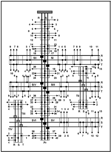
Figure 4 - Real LV Feeders System to Simulation
The FSA algorithm follows the procedure described in section B.1, by replacing the Energy function E to Fff.
The FEPSO algorithm, is described in the flow-chart of Fig. 5. NIterMax is the maximum number of iterations externally defined. It possible to observe the scheme corresponding to PSO, by eliminating the processes called Evolutive Operators and MultiObjetive. By eliminating only the process called MultiObjective, it observe the scheme corresponding to EPSO.

Figure 5 - Flow Chart of FEPSO in Phase Balancing
The parameters used in FSA, are listed below:
a) Initial Temperature: T0 = 1.0;
b) Number of Iteration to the same Temperature: NT=100;
c) Maximum Number of Iterations without improvement of fitness function (stopping condition): nMaxI = 300;
d) Cooling Rate: a = 0.8;
e) Function of Generation of Neighborhood, q(i, j): this identification is making by selection, randomly, of one single phase load, and connecting it in a changed phase.
f) kB Constant (to eq. (6)): kB = 0.00025.
The Fuzzy fitness function, Fff, is evaluated from the results of a three-phase load flow.
The Table 1 shows the results corresponding to application of two metaheuristics (FSA y FEPSO). Table 2 shows the complete results of swapping Phase Balancing for mono-objective PSOs and FEPSO. [S] is the loads power vector [kVA] and [d] the nodes distance vector, respect to substation output [km]. The power factor is 0.85.
Table 1: Results of Metaheuristics FEPSO-FSA-PSO

Table 2: Complete Swaping Phase Balancing Results of Metaheuristics PSO (three simulations) and FEPSO

The model for this application (phase balancing), is static. This implies that the feeders system is analyzed for the worse scenario of the grow load planning, corresponding to the peak of demand for certain period of time (one year, typically). System evolution is not required, because is not a control model. For this propose (static planning) is introduced, in the studies of the electrical distribution systems, a parameter called simultaneity factor of loads. It represents the simultaneous load in the peak of demand. It was considered, in the example, as fs = 0.6. This mean that each value |P + j x Q| (complex power) in [S] vector, Table 2, was multiplied for fs.
The exponential weights can be obtained from the preference matrix between the optimization criteria (Schweickardt and Miranda, 2009). These preferences are certainly subjective, and are expressed in order to Analytical Hierarchy Processes method, proposed by Saaty (1977). Alternatively, these weights can be defined without any previous process, satisfying or not the condition of summatory equal to number of criterias. Follows this way, with an arbitrary choice to emphasize the uncertainties of value, the exponential weights resulting in: pμ(LossT)=pμ(|I[0]|f)=pμ(NC)=3; pμ(vu)=4.
The reference values to form the membership functions to each fuzzy optimization criteria, were results:
[LossTMin=6.94 [kW] ; LossTMax=13.02 [kW] ];
[ I[0]fMin=0.1 [A] ; I[0]fMax=47.6 [A] ];
[NCMin=45 ; NCMax =85], with NC0 = 34;
The parameters used in FPSO, are listed below:
a) Initial Weigths: wI =0.5; wM = wC =2. In PSO are constants;
b) τ and τ' =0.2;
c) Number of Replication for each particle: r = 5;
d) Maximum Number of Iterations without improvement of fitness function (stopping condition): nIterMax =400;
It can observe in the Table 1, the best results reached for the metaheuristic FEPSO, respect to FSA. There are some reason for this: a) FSA exhibit a poor ability to "escape" from local optimal (worse that PSO), when the search space is discrete and the good solutions are very dispersed. In fact, a bootstrapping procedure was necessary to change the membership function of I(Δu) because this index is strict, and the algorithm FSA reached the stopping condition with Fff = 0. The bootstrap, begins with another more flexible membership function, expressed as I(Δu)= μ(vu)# =e-[ξ x Nnot]; 0 < ξ ≤1, where Nnot is the number of terminal nodes with out of tolerance voltage. If, in certain iteration, some solution that satisfy the Eq. (22) is reached, then I(Δu)= μ(vu) (Eq. 22); b) It is no necessary in EPSO, because the self-adaptation introduced by the evaluative operators, allows a self-tuning of weights in the velocity operator. Consequently, this avoid that algorithm to be trapped at some local minimum, or, even worse, at fitness 0; c) In the FSA, even when a bootstrap procedure was introduced, after several simulations, always was reached a local minimum. The solution FSA shown in Table 2, is the best reached in 22 executions of algorithm.
As an example of the evolution of minimized variables (objectives, in the optimization problem), in the Fig. 6 a plot of LossT vs. time computing, t, for both Metaheuristics, FEPSO and FSA, is presented. LossT is the most important parameter to optimize in the classic formulation of phase balancing problem.

Figure 6 - Time and Iterations in FEPSO and FSA Simmulations for Loss Optimization
Additionally, the iterations numbers ItFEPSO and ItFSA are shown at the observation times in the interval [10, 70] [min], until the convergence of two corresponding algorithms is reached. Very similar plots, can be obtained for the other three objectives: |I[0]f|, I(Δu) and NC.
The number of iterations for both metaheuristics, has not significance in a comparative context, because the algorithms's structures are very different.
No "pathological" cases were observed, in which the convergence of both metaheuristics algorithms might be impossible for this application.
As computational cost, (see Table 1) the time computing, t=T, to reach the convergence, is the most representative parameter.
Respect of inherent uncertainties in the loads, the model has considered only the worse scenario of grow demand. But a collection of scenarios of grow demand in a given planning horizon, can be integrated in the analysis of the distribution system, with the aim to define different networks topologies in the LV feeders system. Then, a deterministic simulation for each scenario of grow demand-network topology, is performed. Another way to treat with this kind of uncertainties, can be made by mean of fuzzy sets, considering, as separated fuzzy-variables, the active and reactive power in each load connected to the feeders system (Schweickardt and Miranda, 2007).
III. CONCLUSIONS
The paper offers the following contributions:
- A different meaheuristic approach, based in a variant of PSO Metaheuristics, called FEPSO, that produce very good results in multi-objective combinatorial optimization problems, such as Phase Balancing with only single phase loads in a LV feeders system (and four objectives). It is not possible to solve this problem with mathematical programming techniques.
- A comparison FEPSO vs FSA methaheuristics: this allow to observe the advantages of swarm self-adaptative approach. The swarm intelligence principles, such as cooperation, combined with evolution strategies, seem like and address of metaheuristics toward solution for any combinatorial optimization problem.
- A method to capture and model the uncertainties of value in the optimization criteria, at the same time that are extends to multi-objective decision making, introducing the fuzzy sets modeling, and fuzzy function fitness.
REFERENCES
1. Bellman, R. and L. Zadeh, "Decision-Making in a Fuzzy Environment," Management Science, 17, B-141-164 (1970). [ Links ]
2. Kennedy, J. and R. Eberthart, "Particle Swarm Optimization," Proceedings of the 1995 IEEE International Conference on Neural Networks, Perth, Australia, 1942-1948 (1995). [ Links ]
3. Kirkpatrick, S., C. Gellat and M. Vecchi, "Optimization by Simulated Annealing," Science, 220, 671-680 (1995). [ Links ]
4. Metropolis, N., A. Rosenbluth, A. Teller and E. Teller, "Equation of state calculation by fast computing machines," Journal of Chemical Physics, 21, 1087-1092 (1953). [ Links ]
5. Miranda, V., H. Keko and A. Duque Jaramillo, "EPSO: Evolutionary Particle Swarms," In Advances in Evolutionary Computing for System Design, L. Jain, V. Palade and D. Srinivasan (Eds.), Springer series in Computational Intelligence, 66, 139-168, (2008). [ Links ]
6. Saaty, T., "A Scaling Method for Priorities in Hierarchical Structures," Journal of Mathematical Psycology, 15, 234-281 (1977). [ Links ]
7. Schweickardt, G. and V. Miranda, "A Fuzzy Dynamic Programming Approach for Evaluation of Expansion Distributions Cost in Uncertainty Environments," Latin American Applied Research, 37, 227-234 (2007). [ Links ]
8. Schweickardt, G. and V. Miranda, "A Two-Stage Planning and Control Model Toward Economically Adapted Power Distribution Systems using Analytical Hierarchy Processes and Fuzzy Optimization," International Journal of Electrical Power & Energy Systems, 31, 277-284 (2009). [ Links ]
9. Smith K., Everson J., Fieldsend R., Misra R., and Murphy C., "Dominance-based Multi-objective Simulated Annealing", IEEE Transactions on Evolutionary Computation, 12, pp. 323-342, (2008). [ Links ]
10. Zhu, J., B. Griff and M. Chow, "Phase Balancing Using Mixed-Integer Programming," IEEE Trans. Power Systems, 13, 465-472 (1998). [ Links ]
Received: June 16, 2009.
Accepted: May 11, 2010.
Recommended by Subject Editor José Guivant.

