Strip thickness control in rolling mills using a gain scheduling technique

E. Cavazzana^† and J. Denti Filho^‡

^† Depto. Aut. Industrial, Ifes - Instituto Federal do Espírito Santo, CEP 29901-291 Brazil. erlon@ifes.edu.br
^‡ Depto. Eng. Elétrica, UFES - Universidade Federal do Espírito Santo, CEP 29060-900, Brazil. jdenti@ele.ufes.br

Abstract- This paper proposes a methodology of gain scheduling control for industrial rolling mills to test its feasibility and performance. Two controllers were proposed based on classical gain scheduling techniques acting on gap subsystem to compensate the process disturbances. One of them uses a proposed smoother control action mechanism to improve the process. A local control structure with an integrator in direct path between the controller and the plant was chosen to make the control synthesis more attractive. Optimal quadratic regulator method was used to get the local controllers gains. Simulation results are presented using real industrial data. They showed that the developed gain scheduling controllers are feasible for this process and lead to a less output thickness variations compared with another proposals. It is possible to use the developed control methodology for hot and cold rolling mills.

Keywords- Rrolling Mills; Gain Scheduling Control; Gap Adjustment; Thickness Control.

I. INTRODUCTION

The rolling process of at products involves several subprocess and subsystems, with considerably sophisticated dynamics. They involve, in most cases, nonlinear behaviors (Denti Filho, 1994; Rossomando and Denti Filho, 2006). Several automatic control techniques tested on this process aim to improve the final product quality and costs reduction. The Gain Scheduling technique was tested at coiler and looper subsystems of this process with theoretical data by the same authors and root locus method to get the local controller gains was used (Cavazzana and Denti Filho, 2011a; Cavazzana and Denti Filho, 2011b). Here this technique was evaluated on the gap adjustment subsystem with real industrial data and it was proposed a smother control action mechanism to improve the process. In this case optimal quadratic regulator method was used to get the local controller gains and the results of these two proposals were compared with a fixed gain controller results. The Gain Scheduling technique had never been tested that way before.

A. Gap adjustment subsystem

The main parts of gap adjustment subsystem consist of screws positioners, electric motor, coupling, transmission tree and gears (Fig.1). The rolling mill stands are constituted by four rolls: two work rolls and two back up rolls. The rolls in contact with the strip are the work rolls. The strip is introduced into the gap of the work rolls, which is smaller than the strip thickness. This gap is determined by the screws that set the rolls position. Thus, the control aims to maintain the desired strip thickness acting in this subsystem to adjust the gap and compensate the process disturbances, like changes in entry strip thickness, friction, tensions, temperature and rolling speed.

Figure 1: Rolling mill stand scheme and the gap adjustment subsystem.

This process is developed according to an operation curve c, which relates the rolling load P and the exit thickness h₂. This curve is a function of, called here, operating parameters, like friction coefficient µ, yield stress S, back and front tensions in the strip t₁ and t₂, input strip thickness h₁, rolling speed v_L and so on. The operating point Q depends on the gap opening "g" between the work rolls and the elastic modulus of the rolling mill E_LM, which is represented by the load line r of the system. Thus, disturbances in the operating parameters modify the system curve and consequently the strip thickness output. These disturbances are reflected in the electrical parameters of the machine and can even be used to estimate the process parameters (Marcellos et al., 2009). We can see in Fig. 2 an example of h₂ correction by setting new gap.

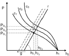
Figure 2: h₂ correction by gap adjustment.

II. SYSTEM MODEL

A. Rolling mill model

Several rolling process models are available in literature. Some models are employed to determine a rolling load P, the rolling torque T_q and the rolling power P_ot, which are related to the strip thickness. The load P can be related to operating parameters, like µ, S, t₁, t₂, h₁, h₂, v_L and θ_t mentioned above. θ_t is the rolling temperature.

The Orowan model (Orowan, 1944) was used in this work because it does not present suppositions for simplification or mathematical approaches. The model was calibrated with real parameters and data kindly given by ArcelorMittal Tubarão, a Brazilian steel making plant, to representate the real process in this work. Equation 1 is used to calculate the rolling load P.

(1)

where w is the strip width, R' is the rolls deformated radius, p⁺(Φ) and p^-(Φ) are the strip radial pressure in input and output areas, α_t is the radial angle of strip and roll, α_N is the angular position in the contact arc where p⁺(Φ)=p^-(Φ). See Fig. 3.

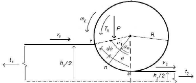
Figure 3: Roll bite geometry.

B. Screw model

Figure 4 shows details of parameters and forces in the screw. The model is constructed as follow:

(2)

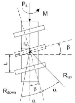
Figure 4: Details of the screw.

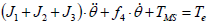
where J₁ is the motor inertia, J₂ the coupling inertia, J₃ the transmission inertia, f₄ the viscous damping coefficient of rolling bearings, T_MS the torque required to move the screw, T_e the torque motor or electromagnetic, θ the angle shaft, the angular speed and the is the angular acceleration.

The required torque to turn the screw may be given by the Eq. 3 (Denti Filho and Lima, 1997).

(3)

where P_s is the resultant forces applied to the screw, d_med the mean diameter of the clamping screw, φ the friction angle in the screw thread, α the turn angle of the screw, µ_s the friction coefficient between the clamping screw and nut, d_g the nut diameter, i the gear reducer ratio and η is the transmission efficiency.

It is possible to notice different dynamics in this system according to the direction of motion. The upward movement is given for tg(φ-α) in the Eq. (3) and the downward movement is given for tg(φ+α).

The translational equation of the system movement is 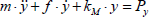, where m is the mass of the set mobile rolls, bearings and load cells, f is the coefficient of viscous damping among stand and roll bearings, k_M the equivalent spring constant of the machine, P_y the resulting forces that act in the screw axis direction, y the linear displacement, the linear speed and the linear acceleration. Notice that P_s and P_y are equals to Lamination Load P.

Since there is an elastic deformation due to the rolling mill efforts involved in the process, the real displacement of the screw is given by:

(4)

To refer all equations to the motor shaft, it is enough to use the relations among θ and y as follow:

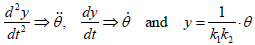	(5)
	(6)

where D_c is the medium gear diameter, D_SF the medium diameter of the thread screw, β the screw thread angle, r_m the medium screw ray, α_s the spiral screw angle.

Thus, the final expression of the requested torque to move the screw T_MS is given by Eq. (7). It is verified in this equation that the T_MS does not change the differential terms coefficients according to lamination load, so it will not change the dynamics response of the linearized system as well as it will not demand different tunings for different rolling mill forces.

(7)

where .

Electrical motor model

The electrical motor used in this system is a DC machine. Its basic equations are described by Eqs. (8) and (9), where e_a=k_vi_a and T=k_ti_a.

	(8)
	(9)

where V_ta is the supply, e_a is the voltage induced at machine armature, L_aq, R_a and i_a are the armature induction, resistance and armature current, respectively, J₁ is the motor inertia, w₁ angular velocity, T_e is the electromagnetic torque and T_MS is the load torque on the shaft.

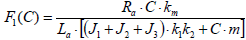
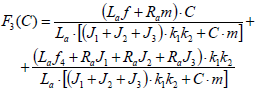
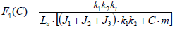
The complete gap adjustment model

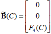
Based on the above equations it was possible to get the complete nonlinear subsystem model below, where , C is given for Eq. (7) and the real displacement is given for Eqs. (4), (5) and (6) where P is derived from Eq. (1). The process was simulated by the Orowan model calibrated with real industrial data.

	(10)
	(11)
	(12)
	(13)
	(14)
	(15)
	(16)
	(17)

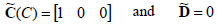
To demonstrate that the linearized process is totally controllable and observable we constructed the controllability matrix and the observability matrix for each C value.

We obtained the matrix rank M_c and the matrix rank M_o equals to the process order for all cases so it confirms this systems are completely controllable and observable. It was assumed that all states are available for measurement in this work.

III. GAIN SCHEDULING CONTROL

The Gain Scheduling control technique has proven to be great useful in nonlinear applications (Rugh and Shamma, 2000) such as: a) The flight control in which the dynamics varies strongly with the speed and the airplane altitude (Stein et al., 1977), b) The industrial process control in which the process dynamics may vary according to the characteristic or the production rate (Doyle et al., 1998) and c) The vehicle control active suspension in which the suspension dynamics varies in accordance with the road profile and others (Tran and Hrovat, 1993). This technique consists of designing linear controllers with different gains for nonlinear systems controlling and associate them in a single nonlinear controller. Thus, different linear controllers are used and each one operates in a certain operation range or, equivalently, it is used only one controller with variable gain to compensate changes in system dynamics and to perform the overall task of the nonlinear system control.

The main advantages of gain scheduling control are the fact that it can be a more simple control method than other control methods for nonlinear systems, and its potential to incorporate the powerful tools and methodologies of linear control in nonlinear systems.

In the classic form of Gain Scheduling project Jacobian linearization of the nonlinear plant on family of equilibrium or operating points is used, being sometimes called scheduling by linearization method. In that way, there are now linear models valid on the neighborhoods of those operating points which are tuned linear controllers. Another way of accomplishment the Gain Scheduling project consists on LPV based forms, in which the plant dynamics are rewritten so that nonlinear time varying parameters are possible to be used as scheduling variables (Leith and Leithead, 2000). The first form has the advantage of using the knowledge of linear controllers widespread in industry, that is why it was chosen to be used in this work.

IV. THE PROPOSED CONTROL

Once the system is nonlinear, the Gain Scheduling project first requests tuning of linear controllers in different operation points. In the present case, this task was accomplished for the two linear models that represent the complete system, where the corresponding controllers were tuned. As the movement direction is related to the direction of rotation motor, it was chosen the parameter as scheduling variable. See Fig. 5.

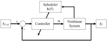
Figure 5: Gain Scheduling scheme.

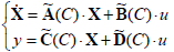
Equation (18) shows the "local"' linear control structure chosen for each C value, where the states are X₁=y, and the control action u is the voltage applied to the motor. This structure was chosen to allow to accomplish, in a relatively easy way, the local controllability evaluation and the tuning of you get the same "local" performance desired for all systems.

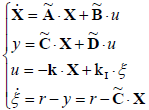(18)

where X is the state vector, y the output, u the control action, and are constant matrices with a defined C value that represent the local linear system, ξ is the integrator output, r the control reference and k is the state feedback gain vector (Ogata, 1996).

Next, the global nonlinear controller was firstly obtained building the gain scheduler mechanism exemplified in Fig. 6 (solid line) for each controller gain, where these gains are functions of the schedule variable . In this figure, the vertical axis represents a generic control gain.

Figure 6: Example of gain scheduling mechanism for a generic control gain.

A. The Improved Controller.

To reduce the occurrence of unwanted vibration and unnecessary equipment waste, it was proposed a smooth transition mechanism for the controller gains to smooth also the variations in the control signal. This mechanism consists of inserting a linear transition region in an area where abrupt changes in gains occur, changing the scheduler function as shown in Fig. 6 (dotted line). The region transition value chosen for this work is in the range between -10 rad/s and +10 rad/s of and this was implemented using "lookup tables" in Matlab® software, a Mathworks Inc. product.

B. Tuning method.

Optimal Quadratic Regulator method was used in this work to get the controller gains. This method is based on the performance minimization index J shown in Eq. (19).

(19)

where Q is a Hermitian positive definite matrix or real symmetric or positive semidefinite and R is a Hermitian matrix or real symmetric positive definite. The optimal gain matrix is given by k=R^-1B'P and the matrix P must satisfy Eq. (20) called Ricatti reduced matrix equation.

(20)

Thus, the optimal control law is linear and becomes .

Due to the existence of the integrator in the structure, the following transformation is necessary before applying the LQR method:

(21)

This new system is also completely controllable type, because it has rank n+1. So, the matrix of controller gains is given by .

R and Q matrices used in this work are shown in Eq. (22) and (23) and they where chosen to obtain fast control results with reasonable control action.

	(22)
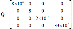	(23)

These matrices were used in all controllers.

V. RESULTS

Real data from a real hot rolling mill process were used to obtain the control results. These data present process disturbances, like variations on the input strip thickness, temperature, rolling speed and others. Figure 7 shows the measurement signal of the real process to exemplify a disturbance, where there is a input thickness reduction around 80s.

Figure 7: Input strip thickness.

Figure 8 shows the strip exit thickness as control result of the first Gain Scheduling controller. It was verified that the control system maintains the setpoint of 21mm even when process disturbances occur. The control system quality was quantified using the Mean Absolute Percentage Error (MAPE) and in this case it was 0.0569.

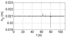
Figure 8: Exit strip thickness.

Figure 9 shows the system control action in zoom view. The noisy appearance reflects the abrupt variations of the gains.

Figure 9: Control action in zoom view.

The rolling mill load shown in Fig. 10 is the result of several process disturbances such as temperature reduction around 60s, reduced input thickness around 80s, rolling mill speed variations at the same time and others.

Figure 10: Rolling mill force.

Figure 11 shows the system gap. This also reflects the elastic machine deformation.

Figure 11: System gap.

Performing the same test with the improved controller (second controller) the control action become smoother as expected. It is possible to see in Fig. 12 a zoom view at the achieved result. The MAPE in this case was 0.0602.

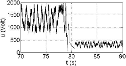
Figure 12: Smoother control action in zoom view.

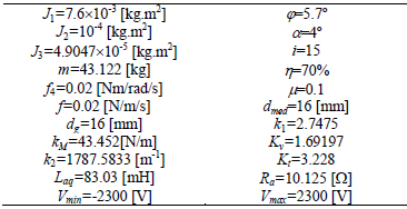
Table 1: Constants used in the models.

The last test consisted of accomplishing the control without scheduling to compare the results. In other words a controller (third controller) was tuned with fixed gains using the same control structure as the first one. It was chosen the upward movement and it was tuned a single controller for all system using the same R and Q matrices presented. In this case the MAPE obtained was 0.0622.

In all cases we verified that the error of the output strip thickness was around 25mm, better than another proposals like in Rossomando and Denti Filho (2006).

The guarantees of stability and performance were inferred in all cases by extensive simulations across all operation range, in different situations, values and process real data.

VI. CONCLUSIONS

This paper presents a Gain Scheduling control methodology for industrial rolling mills. Two strip thickness controllers by gap adjustment where proposed based on classical methods. To reduce the possibility of unwanted vibrations and unnecessary waste on the equipment it was developed a smoother control action mechanism of scheduled gains, being this an improvement of the first controller. A great advantage of this type of controller is the use of the linear controllers knowledge widely used in industry.

The models presented in this work were calibrated with measured data from a real hot rolling process and constructed with parameters kindly provided by ArcelorMittal Tubarão, a Brazilian steel making plant. During the gap setting subsystem modeling it was observed that the rolling load P does not change the system dynamics and therefore it does not interfere with scheduled controller gains. The variation of the dynamic system is due exclusively to the direction of the cylinders movement, which can be represented all system by two different linear models. Each model requests a linear tuning controller and in this work it was proposed a scheduling using the variable as scheduler variable.

It is important to stand out that the use of the integrator in the direct path between the controller and the plant, in the "local" controller's structure adopted, simplifies the Gain Scheduling design, making possible to reduce system installation and maintenance costs.

The control tests results using real data of a real hot rolling mill process demonstrated the proposed control viability. The tests have shown that the first Gain Scheduling controller MAPE was 8.52% better than the fixed gains controller performance. The improved controller was 3.22% better but its main advantage was the smoothing of control action. The control error of the strip thickness was around 25 mm, better than traditional methods in literature. Due the fact that P does not change the system dynamic behavior, this methodology is valid for hot and cold rolling mills.

REFERENCES
1. Cavazzana, E. and J. Denti Filho, "Modelagem, Simulaςão e Controle da Velocidade Tangencial em um Sistema de Bobinamento de Tiras de Aςo," 10th Conf. Brasileira de Dinâmica, Controle e Aplicaςões, 627-630 (2011a).         [ Links ]
2. Cavazzana, E. and J. Denti Filho, "Modelagem, Simulaςão e Controle de um Sistema de Tensionamento de Tiras de Aςo via Abordagem Gain Schedulling Clássica," 10th Conf. Brasileira de Dinâmica, Controle e Aplicaςões, 747-750 (2011b).         [ Links ]
3. Denti Filho, J. and L.E.M. Lima, "A New Theoretical Exit Thickness Control Model for Rolling Process," Int. Conf. on Modelling, Identification and Control, Anaheim-Calgary-Zürich, 1, 490-493, (1997).         [ Links ]
4. Denti Filho, J., Um método de controle dinâmico de laminadores reversíveis, UFMG, Brazil (1994).         [ Links ]
5. Doyle, F.J.I., H.S. Kwatra and J.S. Schwaber, "Dynamic Gain Scheduled Process Control," Chemical Engineering Science, 53, 2675-2690 (1998).         [ Links ]
6. Leith, D. and W. Leithead, "Survey of gain-scheduling analysis e design," Int. Journal of Control, 73, 1001-1025 (2000).         [ Links ]
7. Marcellos, N.S., J. Denti Filho and G.C.D. Souza, "Strip thickness estimation in rolling mills from electrical variables in AC Drives," Latin American Applied Research, 39, 353-359 (2009).         [ Links ]
8. Ogata, K., Modern Control Engineering, Prentice Hall Inc, third edition (1996).         [ Links ]
9. Orowan, E., "The Calculation of Roll Pressure in hot and Cold Rolling," Proc. Inst. of Mechanical Engineers, 150, 140-167 (1944).         [ Links ]
10. Rossomando, F.G. and J. Denti Filho, "Modelling and control of a hot holling mill," Latin American Applied Research, 36, 199-204 (2006).         [ Links ]
11. Rugh, W.J. and J.S. Shamma, "Research on gain scheduling," Automatica, 36, 1401-1425, (2000).         [ Links ]
12. Stein, G., G.L. Hartmann and R.C. Hendrick, "Adaptive Control Laws for F-8 Flight Test," IEEE Trans. on Automatic Control, 22, 758-767 (1977).         [ Links ]
13. Tran, M.N. and D. Hrovat, "Application of Gain-Scheduling to Design of Active Suspensions," 32nd IEEE Conference on Decision and Control, San Antonio, TX, USA, 1030-1035 (1993).         [ Links ]

Received: August 22, 2012
Accepted: December 13, 2012
Recommended by Subject Editor: Jorge Solsona