REGULAR PAPERS

Mg-Cu alloys: A Monte Carlo Simulation of structural and thermodynamic properties

Hojvat de Tendler, R.^1*; Fracchia, R. M.²; Pepe, M. E.³; Lavrentiev, M. Yu⁴; Soriano, M. R⁵

¹ Instituto de Estudios Nucleares, Centro Atómico Ezeiza, Comisión Nacional de Energía Atómica, Avda. del Libertador 8250, C1429BNP Buenos Aires, Argentina,
Fax: +54 11 6779 8452, E-Mail: hojvat@cae.cnea.gov.ar
² Dpto. de Qca. Inorgánica, Analítica y Químico Física, FCEyN, UBA. Pab. II, Cdad. Universitaria, C1328EHA Buenos Aires, Argentina.
³ Servicio de Informática y Comunicaciones, Centro Atómico Constituyentes, Comisión Nacional de Energía Atómica, Avenida del Libertador 8250, C1429BNP Buenos Aires, Argentina
⁴School of Chemistry, University of Bristol, Cantock’s Close. Bristol BS8 1TS, UK
⁵ Departamento de Ingeniería Química, Facultad Regional de Buenos Aires, UTN, Medrano 951, C1179AAQ Buenos Aires, Argentina

Received March 2^nd, 2005. In final form June 28, 2005

Abstract
Different properties of Mg-Cu alloys have been studied by using Monte Carlo (MC) simulation and embedded-atom method (EAM) interatomic potentials. The interatomic potentials were derived by fitting to properties of crystalline phases. The pair distribution function g(r) has been calculated showing that a crystal, an amorphous solid, a supercooled liquid, or a liquid can be produced. The RSD (root mean square displacements) have been calculated for the same temperatures and compositions. The Radial Distribution Function (RDF) let us carried out structural analyses. We have been able to reproduce the experimentally measured structural properties of the liquid with potentials fitted to the solid state. The chemical potential is obtained from calculation and thermodynamic properties are derived. Examples studied are the free energy of mixing for liquid and solid alloys. The integral excess free energy, the thermodynamic activities and the activity factors of Mg and Cu were calculated. A good agreement with experimental results is obtained for the theoretical calculations.

Resumen
Diferentes propiedades de aleaciones de Mg-Cu se estudiaron usando simulación de Monte Carlo y el método del átomo implantado de potenciales interatómicos(EAM). Los potenciales interatómicos fueron derivados por ajuste a las propiedades de fases cristalinas. La función de distribución de pares g(r) calculada indicó que un cristal, un sólido amorfo, un líquido sobreenfriado o un líquido pueden ser producidos. The RSD ha sido calculado para las mismas temperaturas y composiciones. La función de distribución radial (RDF) permitió realizar análisis estructurales. Se reprodujeron las propiedades estructurales medidas experimentalmente del líquido con potenciales ajustados al estado sólido. El potencial químico se obtuvo por cálculo y se derivaron propiedades termodinámicas. Se estudiaron la energía libre de mezclado para líquidos y aleaciones sólidas. Se calcularon el exceso de energía libre integral, las actividades termodinámicas y los factores de actividad de Mg y Cu. Se obtuvo una buena concordancia entre los resultados experimentales y los cálculos teóricos.

Introduction
Knowledge on structural and thermodynamic properties of alloys is of interest for practical applications. There are previous calculations on Mg-Cu system. A description of different CALPHAD (Computer Coupling of Phase Diagrams and Thermochemistry) method calculations has been summarised by C. A. Coughanow et al. [1]. Different models have been used previously to calculate the enthalpy of mixing of liquid Cu-Mg alloys, Agrawal [2] et al. consider an statistical thermodynamic approach, Sommer [3] et al. used two different models, an associated one and the Miedema model [4]. The goal of this theoretical study of Mg-Cu alloys is the calculation of structural and thermodynamic properties of liquid and solid phases using Monte Carlo (MC) simulation and embedded-atom method (EAM) interatomic potentials which is a modern potential regularly used for metals.
In CALPHAD methods an optimized set of thermodynamic functions are obtained to calculate the Mg-Cu phase diagram and thermodynamic properties, enthalpy of mixing, Gibbs energies of the liquid and the solid phases. One of us made a theoretical calculation of the amorphous alloy range of the Mg-Cu system using the Miedema model [5]. In this work the authors reproduce the amorphization range, the instability of the solid solution from pure Mg up to near the pure Cu end, the small solid solubility range in fcc Cu, and the role played by the intermetallic compounds on defining the amorphization range. Most of these works show a good fit to experimental data. Atomistic calculations have been reported on Mg-Cu metallic glasses [6,7]. Atomistic methods provide a link between the atomistic scale and the macroscopic mechanical, thermodynamic and chemical behaviour of matter. The use of these methods for metallic alloys is a real challenge and is highly desirable to try them and prove their ability to reproduce and predict thermodynamic behaviour. Great efforts have been, and still are, dedicated to the development and improvement of potential energy functions. This work shows good results for structural and thermodynamic properties.
The EAM, a semiempirical interatomic-potential method, has been extensively applied in the study of crystalline metals and alloys [8]. A very good agreement between EAM simulations and experimental measurements has been found in a previous study of liquids of fcc transition metals that was performed by Foiles [9]. Nowadays the EAM has been widely used to study the structural, thermodynamic and dynamic properties of elemental metallic liquids and glasses.
The existing experimental results make it desirable to include new theoretical evaluations that may reproduce more satisfactorily their behaviour. This is what we will tackle in this work. A number of authors have measured thermodynamic properties of solid and liquid Mg-Cu alloys experimentally and the results have been critically assessed by Hultgren [10]. Subsequently Juneja et al. [11] studied the thermodynamic behaviour of liquid Mg-Cu alloys and compounds by a modified form of the boiling-temperature method, which was not previously used for the studies of these alloys. Experimental studies by Lukens and Wagner [12] analyse the structure of Mg-Cu liquid alloys. Sommer et al. [13] presented thermal properties of Mg-Cu glasses and Mg_85.5Cu_14.5 liquid and crystalline alloy.
The phase equilibrium diagram has been critically evaluated by Nayeb-Hashemi et al. [14]. They described that the equilibrium phases of the Mg-Cu system are the liquid, the Mg terminal solid solution (hcp) which has a restricted solubility of Cu in Mg; and the terminal (fcc) solid solution of Mg in Cu with a maximum solid solubility of 6.93% at Mg. Two intermetallic compounds exist, the orthorhombic stoichiometric Mg₂Cu and the non-stoichiometric MgCu₂ fcc, C-15 type structure. Both of them melt congruently at 568 °C and 797 °C, respectively. Mg-rich metallic glasses were obtained by Sommer et al. [13] and Kempen et al. [15] by rapid quenching from the liquid state. Glass formation occurs from 9 to 42 at. % Cu and the region of complete glass formation 12 to 22 at. % Cu appears around the deep eutectic (14.5 at. % Cu and 485 °C) L<—> Mg₂Cu + (Mg). In our simulation we examine some of the equilibrium phases, the liquid at 827°C (1100 K), Mg-rich hcp and Cu-rich fcc solid solutions and the two existing intermetallic compounds Mg₂Cu and MgCu₂.
The thermodynamic and structural properties are studied with MC simulations at constant pressure and temperature. Different temperature calculations were performed. The different arrangement of atoms is represented with the exchange of atoms located in crystallographically unequivalent positions. The environment of each atom and the local structure and movements are then taken into account. The structural movement that accompanies any exchange of an atom reduces considerably the energy associated with any such interchange. This approach was previously used in the study of rhodium-palladium solid solution [16]. We have checked the convergence of the calculated thermodynamic properties by performing MC simulations using a box-size of 256, 512, 864 and 2048 atoms. The interatomic potentials were derived by fitting to properties of crystalline phases. The experimental data used in the fitting are the elastic constants, sublimation energy and lattice parameter. One of our goals is to study the accuracy of results for liquids when using potentials derived from solid state properties.
Method and potentials are described in the next section. Calculated properties are presented and compared with experimental available data in the Results and Discussion Section. At the end, our conclusions are summarised.

Method
A. Interatomic Potentials
In the EAM [17-19] the lattice static energy per unit cell can be written as:

Primes on summations in this and subsequent equations indicate that terms with r_ij = 0 are excluded. F_i(r_i) is negative and represents the energy of “embedding” atom i in the electron density r_i created by all other atoms in the crystal, and f_ij(r_ij) is the core-core repulsion between atoms i and j , assumed to depend only on the type of the atoms and the distance between them. The electron density r_i is assumed to be the sum of the electronic densities of all other atoms at the nucleus of atom i :

The electron density created by atom j at a distance r_ij , f_j(r_ij), is assumed to be isotropic about j.
The computational cost is not much higher than that when using only two body potentials. Although angular contributions are not included explicitly, account is taken of many body contributions to the crystal energy through the embedding function.
In this work we represent the electronic densities, the two body potentials and the embedding function with simple analytical functions. For the electronic densities we use exponential functions:

with different parameters D_j and z_j for each metal (j = Cu, Mg). The embedding energy (equation 1) is given by

with different parameters C_j again for Cu and Mg. The repulsive potential in equation (1) is also given a simple form,

where A_ij and s_ij are different for each type of interaction (Cu-Cu, Mg-Mg, Cu-Mg). A cutoff of 6 Å was used for both electron densities and repulsive potentials.
For pure Cu five parameters need to be determined: D_Cu , z_Cu , A_CuCu , s_CuCu, and C_Cu. Because the energy of any given configuration depends only on [(C_Cu).(D_Cu)^1/2] and not on the separate values of C_Cu and D_Cu, only four of these parameters can be determined by fitting to properties of the pure metals. Without loss of generality we take . The remaining four parameters are fitted so as to reproduce the experimental lattice parameter, sublimation energy [20] and elastic constants [21] of pure Cu. In table 1 we show the experimental data used in the fitting together with the values obtained from the present model. With this simple model it is not possible to reproduce the experimental values exactly. The same procedure was followed for Mg with experimental data taken from Kittel [20] and Simmons et al. [22]. Although the parameters C_Cu and C_Mg can be taken as 1 for the pure metals, the energies of Cu-Mg alloys depend on their relative values. Here, we take C_Cu = 1 while the parameter C_Mg, together with the cross interaction parameters A_CuMg and s_cuMgare fitted to reproduce the experimental values [23] of the lattice parameters a and the formation enthalpy of CuMg₂. Experimental and calculated values are given in Table 1. In Table 2 we collect together the parameters of the present potential. The fitting was performed using the computer code EAMLD [24].

Table1. Experimental data used to determine the model parameters and corresponding calculated values.

Table 2. Parameters of the potential model used in this work.

B. Monte Carlo
Our starting point was a MC simulation at constant temperature and pressure. Vibrational effects are taken into account by allowing random moves of randomly selected atoms. Both atomic coordinates and cell dimensions are allowed to vary during the simulation. During one step of the MC simulation an atomic coordinate or a lattice parameter is chosen at random and altered by a random amount. To determine whether the change is accepted or rejected, the usual Metropolis algorithm [25] is applied. The maximum changes in the atomic displacement and the lattice parameter are governed by the variables r_max and n_max respectively. The magnitudes of these parameters are adjusted automatically during the equilibration part of the simulation to maintain an acceptance/rejection ratio of approximately 0.3.
In the MC calculations each step thus comprises either an attempted atom movement or a change of size of the simulation box. The MC calculations thus almost always sample only one atom arrangement, the initial configuration which is chosen at random. In order to sample different configurations in an efficient way we have carried out Monte Carlo exchange simulation (MCX). Details of this technique were already described [26]. Detailed balance is achieved, at any stage of the simulations by deciding whether to carry out an atom displacement, a cell distortion or an exchange, at random with a probability of N: 1 : 1, respectively, where N is the number of atoms in the simulation box. Most of our simulations were carried out using a unit cell with 256 atoms and 2 x 10⁷ steps.
To speed up the sampling of configuration we have applied the biased sampling technique [27]. In our exchange bias MCX, instead of considering a single trial exchange, a set of trial exchanges is picked at random, and one of this set is chosen [28].

Figure 1: Enthalpy of pure Cu at temperature T (K) relative to its standard state at 298.15 K. Thick +: experimental data [10] Calculated values, this work, thin +: starting from perfect crystal, x: starting from liquid Cu simulated at 1773 K, o: starting from a half liquid-half solid cell. Lines joining thick + symbols are included only as an eye-guide. 1: experimental T of melting [10], 2: calculated T of melting (this work).

Figures 2a and 2b: pair distribution function (Figure 2a) and root square distance (Figure 2b) for pure Cu simulated in this work at different temperatures starting always from a simulation cell containing a liquid-like configuration.

Figure 3: Molar volume of our calculated liquid (o) and crystal phases (+) of pure Cu, as well as values calculated in this work from experimental results on thermal expansion [29] and lattice parameter [30] data (x)

Results and Discussion
A. Pure Cu and Mg
Figure 1 shows the variation with temperature T (K) of the enthalpy of pure Cu relative to its standard state at 298.15 K, (H_T-H_st). The experimental values selected by Hultgren et al. [10] and the values calculated in this work are represented showing the very good agreement that exists between theory and experiment. The liquid-solid transition can be seen in the variation of the enthalpy as a function of temperature, with the characteristic jump in enthalpy at the melting point. This characteristic jump can also be seen in Figure 3, representing volume (V) vs T. This behaviour will be described below. The experimental temperature of melting of pure Cu is 1356.55 K [10], which is indicated in Figure 1. The calculated values of H_T-H_st agree with the experiment [10] when starting from half liquid-half perfect crystal cells (composite cells) and from perfect crystal cells. The value of T_f from simulations performed starting from the initially perfect crystal is 1466 K. This value has been estimated by simulating at various temperatures around 1466 K, separated 10 degrees increments (Figure 1). The enthalpy of melting from the simulation at 1466 K is 11.6 kJ/Mol.K and the measured enthalpy of melting 13.05± 0.83 kJ/Mol.K.
When simulations start from a liquid configuration previously simulated at 1773 K a liquid is obtained even at 1173 K. This behaviour could be justified considering that interatomic potentials were obtained by fitting properties of crystalline phases. Below this temperature a supercooled liquid (1073 K) is obtained or solidification occurs into thermally disordered crystals (873 K and 973 K), as Figure 2a and 2b show. In Figure 2a the pair distribution functions g(r) calculated at these temperatures are depicted, showing that crystals, a supercooled liquid, or an amorphous solid have been produced, the pair distribution function provides an insight into the corresponding structures. A crystalline system shows peaks broadened by thermal fluctuations, for the liquid the long–range order diminishes with distance and the split of the second nearest neighbour peak is present in the amorphous, we can see these characteristics in Figure 2a. In Figure 2b the root mean square displacements (RSD) calculated for the same temperatures show the liquid, the amorphous and the crystal.
Figure 3 shows the variation of the molar volume of pure Cu with temperature. The discontinuity in the variation of the calculated values with T corresponds to the liquid-crystal transition. For this figure we have worked out the experimental values of the molar volume from DL/L₀ % selected by Touloukian et al. [29] and adopting as L₀ the experimental lattice parameter of Cu compiled by King [30].

Figure 4: Cp as a function of T (K). experimental values: +:crystalline and liquid Cu [10], D: superheated Cu crystal [31]; ‚: simulated values and their error bars, this work. -: experimental T_f [10], - - -: calculated T_f, this work.

In Figure 4 the simulated C_p values for pure Cu are represented against temperature, the calculations were done for crystalline and liquid Cu. Around fusion temperature C_p values follow the same behaviour as experimental data, some data increase with temperature whereas other present a constant value. Errors were estimated as the square root of the value of the variance and are represented in the same Figure. The variation of the experimentally measured C_p with T (K) included in this Figure for crystalline and liquid Cu were taken from Hultgren [10] and for solid Cu superheated above its melting temperature from Janaf tables [31].

Figure 5: Pair distribution function g(r) for pure liquid Cu at four different temperatures. - —— : calculated values (this work), + : experimental values [32]

The experimental pair correlation function g(r) has been tabulated by Waseda [32] for liquid Cu at 1873 K, 1773 K, 1573 K and 1423 K. In Figure 5 the very good agreement of the g(r) curves that have been calculated in this work is shown through the comparison with the experimental g(r) points [32]. The g(r) curves have the typical shape for liquid metals at every temperature in this figure. At 1873 K, 1773 K and 1573 K liquid Cu has been simulated from pure fcc Cu perfect lattice. To simulate the liquid at 1423 K the starting configuration was liquid Cu at 1773 K. When starting from the perfect crystal a crystal is obtained at 1423 K (this result is shown in Figure 1). Figure 6 shows the same comparison for pure liquid Mg at 953 K, which has been simulated starting from the perfect fcc crystal of pure Mg. Table 3 contains the measured [33] and calculated (this work) values of the structural characteristics of the main peaks of g(r) for pure Cu at 1423 K and pure Mg at 953 K.

Figure 6: Pair distribution function g(r) for pure liquid Mg at 953 K. The solid line shows the function calculated in this work. •: experimental values taken from [32]

Table 3: Comparison between calculations (this work) and experiment [33]. Structural information on the main peaks of g( r ) for liquid Cu and Mg near their melting points. Average interatomic distance = (atomic volume/Avogadro number)^1/3

Pure Mg is hcp structure but the alloys were modelled as hcp only at 300K, and will be presented in next section. For pure Mg hcp at 300K we have obtained the lattice parameters (a =3.230 Å and c=5.271Å) in good agreement with experimental data (table 1). Other calculated properties were C_p =26.538 kJ/mol and the coefficient of linear thermal expansion (8.37 K^-1) both near experimental data (24.895 kJ/mol and 8.2 K^-1).

B. The Alloys
B1. Structure
The structure of liquid Cu, Mg and Mg-Cu alloys has been experimentally studied by Lukens and Wagner [12]. They used X-rays as a radiation probe to evaluate the interference functions (or structure factors) for pure Cu at 1373 K, pure Mg at 973 K and Mg-Cu alloys with 49, 66 and 86 at % Mg at temperatures about 50 °C above the liquidus (958 K for the 49 at % Mg alloy and 873 K for the 66 and 86 at % Mg alloys). They determined the positions of the first peak (r₁) and of the second peak (r₂) in the reduced partial distribution function that they assumed composition independent and in the total distribution function G(r) and the coordination numbers h from the radial distribution functions (RDF(r)). As the coordination numbers decrease to a minimum with the increasing Mg content of the alloy, the existence of short-range order in the liquid is assumed by Lukens and Wagner [12]. We have simulated pure liquid Cu and Mg and the liquid alloys with 49, 66 and 86 at % Mg at the temperatures of the experiment. We have calculated the pair distribution (or probability) function g_ij(r) (i, j: Mg, Cu). From these we obtained the reduced partial distribution functions:

where r₀ is the macroscopic atomic density of the material. To calculate the reduced total distribution function we have used:

With

w_ij obtained from X-ray scattering experiments are for Cu-49at%Mg alloy [12] and we have adopted these reported values for the corresponding alloy. We have calculated wij for all the alloys and for the pure metals from the coherent scattering length for neutrons scattering in pure Cu and pure Mg [34]. The radial distribution function is:

and the area under its first peak gave us the coordination number h. We did not find meaningful differences in G(r) and RDF(r) when using neutron or X-rays scattering factors. In this work the area under the first peak has been calculated by considering the minimum after the first peak as the cutoff point. Figures 7 and 8 show the curves G(r) and RDF(r) calculated in this work. Table 4 shows the values of the position of the first and second peak maxima of G(r) for the pure metals and the alloys, as obtained in the present work and comparison with experiment. The results of the simulation show also a minimum in h as a function of Mg contents, it should correspond to the existence of short range order in the alloy.

Figure 7: Reduced total distribution functions of the liquid Cu-Mg alloys simulated in this work. They compare with the experimental results shown in Figure 3 from reference [12].

Figure 8: Total radial distribution functions of the liquid Cu-Mg alloys simulated in this work. They compare with the experimental results shown in Figure 5 from reference [12].

Table 4. A comparison between simulation (this work) and experiment [12] for the pure liquid metals Cu and Mg and for Mg-Cu alloys: Positions of the first and second peak maxima of G(r) (r₁ and r₂). Coordination numbers h calculated from the radial distribution function.

B.2. Thermodynamics
Simulations were performed using semigrand-canonical [28] ensemble to calculate the difference in chemical potential of Mg and Cu atoms. In this method one specie, Cu, is converted in another, Mg, and the resulting potential energy change DU_Mg/Cu determined. This is related to the change in chemical potential Dm by

Each fifth step, on average, we evaluate the energy associated with the conversion of a randomly chosen Cu atom to Mg, DU_Mg/Cu, and as the simulation proceeds determine the average value of the exponential in equation (10). The change of Mg into Cu is only considered but not actually performed, the configuration remains unchanged after evaluating DU_Mg/Cu.
We first consider Gibbs free energy for Mg-Cu liquid alloys at 1100 K. Figure 9 shows our calculated values of chemical potential differences for Mg-Cu liquid alloys at 1100 K.
Simulated values of Dm/kT have been fitted by

Integration of equation (11) with respect to the Mg atom fraction (x(Mg)), and the use of the pure liquid component metals at 1100 K as references (liquid Mg and supercooled liquid Cu) gives the Gibbs energy of mixing of the alloy at 1100 K:

It is represented in Figure 10a together with the experimental values selected by Hultgren [10] and with later measurements by Juneja et al. [11]. The minimum of the calculated curve is located around x(Mg) = 0.6 near its location at x(Mg) = 0.5 in the experiment, which is a meaningful coincidence. The agreement with the experimental data improves, as expected, near the pure metals, towards the extremes of the curve.

Figure 9: Calculated values of chemical potential differences (Dm/kT) as a function of Mg atomic fraction (x(Mg)), for Mg-Cu liquid alloys at 1100K, this work.

Figure 10b shows the separation from ideality of the integral free-energy at 1100 K, that is the excess free-energy. D^EG_m calculated from simulated values of Dm/kT represented in figure 10b is compared with D^EG_m free-energy calculated from experimental measurements selected by Hultgren [10] and from measurements of Mg vapour pressures done by Juneja [11]. The minimum of modelled curve is only slightly shifted towards richer in Mg values. The so-called experimental values for mixing free Gibbs energy are not direct measurements but entail the use of models including excess functions. The difference between our model calculation and the other authors results in Figures 10 does not show which one is better.
Figure 11a shows our calculated values of the thermodynamic activities of Mg and Cu at 1100 K together with the experimental data reported in [10] and [11]. The large negative deviations from ideality exhibited in the experimental curves are more pronounced in our calculations of the activity of Mg and less pronounced in the calculated activity of Cu. Figures 11b and 11c show the activity coefficients g(Mg) and g(Cu) plotted against (1-x(Mg))2 and (1-x(Cu))2, respectively. Although in both Figures the plot can be fitted by two terminal straight lines and a central curve region, as it is expected for metallic systems [11] only in the Cu-rich extreme the calculated straight line for the modelled alloy coincides with the straight lines calculated from the experimental results.

Figure 10: Mg-Cu liquid alloys at 1100K a: — : curve of Gibbs free-energy of mixing, calculated in this work, experimental values selected by Hultgren [10] (+) and measured by Juneja [11] (x). Experimental errors ( I ) limited by ( —- ) labelled H [10] and labelled J [11]. b: — : curve of Gibbs excess free-energy, calculated in this work, experimental values selected by Hultgren [10] (+) and measured by Juneja [11] (x). Experimental errors ( I ) limited by ( — ) labelled H [10] and labelled J [11].

figura 11a

figura11b

figura11c
Figure 11: Liquid Mg-Cu alloys at 1100 K. a: Activities of Mg and Cu; x(Mg): Mg atomic fraction. — : calculated values, this work; (a),- - -: Hultgren et al. [10]; (b),.... : Juneja et al. [11]. b and c: curves of the activity coefficients calculated in this work g(Mg) and g(Cu) plotted against (1-x(Mg))² and (1-x(Cu))², respectively. Experimental g(Mg) and g(Cu): + [10], x[11]. b: Cu-rich extreme, terminal straight line - - - (this work), — [11]. c:— Cu-rich extreme, terminal straight lines, this work and references [10] and [11].

Figure 12: Enthalpy of mixing of Mg-Cu alloys at 1100 K. o and —: calculated values (this work), + and error bar limited by -: Hultgren et al. [10], x and error bar limited by •: Juneja et al. [11]

In Figure 12 the calculated and experimental values of heat of mixing are shown and the calculated and experimental values of entropy of mixing and excess entropy are represented in Figure 13. The calculated heat of mixing is more negative than the experimental values, this behaviour leading to the high values of mixing and excess entropy as compared with the experiment (Figure 13). The asymmetry of the heat of mixing curve is slightly shifted towards 0.6 Mg at. fr. whereas the experimental data shows a minimum between 0.4 and 0.5 Mg at. fr. Nevertheless, the differences between experimental and calculated heat of mixing values in this work are much smaller than those presented by other authors, using also EAM model, for a different system [35]. The calculated curves of entropy of mixing and excess entropy are within the error bars determined at x=0.5 by Hultgren et al. [10] and by Juneja et al. [11], but the departure from ideality is greater for the simulated alloys than in the experiment.
The free-energy curves for the metastable fcc and hcp solid solution at 300 K have been calculated. Figure 14 shows the calculated values of Dm/kT fitted to the cubic polynomia (equation 11) as a function of the Mg atomic fraction for the Mg-Cu fcc and hcp crystalline alloys at 300 K. In Figure 15 the alloy free energy of mixing referred to the free energy of the pure metals at the simulation temperature are represented at 300 K. The free-energy was obtained by using equation 12. Hcp is more stable than fcc from 0.2 at % Mg to pure Mg. From pure Cu up to 0.2 at % Mg the fcc solid solution is relatively more stable than the hcp solid solution. By extrapolating the solvus curve at the rich-Cu end of the assessed phase diagram [14] down to 300 K an experimental solid solubility limit of approximately 0.03 at % Mg in fcc Cu is obtained. The g(r) curve for the thermally disordered metastable fcc crystalline solid solution at 300 K is shown in Figure 16 for 60%at. Mg.

Figure 13: Molar entropy of mixing and molar excess entropy of Mg-Cu liquid alloys at 1100 K. Molar entropy of mixing: —: calculated function; ‚ and I limited by –: experimental values and error bar due to Hultgren et al. [10]; rombo and dashed I limited by ^: experimental values and error bar due to Juneja et al. [11]. Excess molar entropy: - - - curve: calculated function; +: experimental values due to Hultgren et al. [10], x and dashed I limited by ^: experimental values and error bar due to Juneja et al. [11].

We have simulated the solid solution and the liquid alloy at 1173 K by using half liquid-half solid cells. From 1 at % Mg alloys up to 2 at % Mg alloys simulations gave a crystal and for the other compositions (from 3 at. % Mg up to 90 at. % Mg) gave the liquid alloy, as it is expected from the phase diagram [14]. We obtained Dm/kT for the solid and for the liquid phases. Fitting with equation 11, and integrating (equation 12), we have obtained D^MG_s and D^MG₁, referred respectively to the mixture of the pure solid metals and the pure liquid metals [28]. Then, we added to D^MG₁ a term that is the sum of the free-energy differences between the supercooled liquid and the crystalline states of the pure components DGⁱ_l-s, (i=Cu, Mg) weighted by their respective concentrations. We have calculated DGⁱ_l-s, using Turnbull approximation [36]:

Adding this term, the process of obtaining the liquid alloy at 1173 K can be described as follows. Pure crystalline metals melted at 1173 K mix giving the liquid alloy at this temperature. By adding this term both free-energies are referred to the mixture of pure crystalline metals. Curves are shown in Figure 17. Drawing the common tangent to both curves in the Cu-rich extreme we have obtained pure Cu in equilibrium with the Cu-10 at % Mg liquid alloy at 1173 K. The experimental concentrations taken from the phase diagram are 3.5 at % Mg for the solid solution in equilibrium with a 13 at % Mg liquid alloy at 1173 K.

Figure 14: Mg-Cu alloys, calculated chemical potential differences fitted by equation (11) . + and ---: metastable fcc solid solution at 300 K; x and ---: metastable hcp solid solution at 300 K.

B.3. The Compounds
The non-stoichiometric MgCu₂ fcc, C-15 type structure and the orthorhombic stoichiometric Mg₂Cu compounds have been simulated at 300 K. Experimental MgCu₂ lattice parameter and enthalpy of formation [23] were used to adjust Mg-Cu interactions (see Method above) using the EAMLD computer code. The experimental [37] and calculated lattice parameters of both compounds are shown in Table 5.

Figure 15: Mg-Cu alloys, free-energy of mixing. ---: metastable fcc solid solution at 300 K;- .- . : metastable hcp solid solution at 300 K.

Figure 16: Mg 60 at.%-Cu thermally disordered crystalline alloy simulated in this work at 300 K and its calculated partial pair distribution functions.

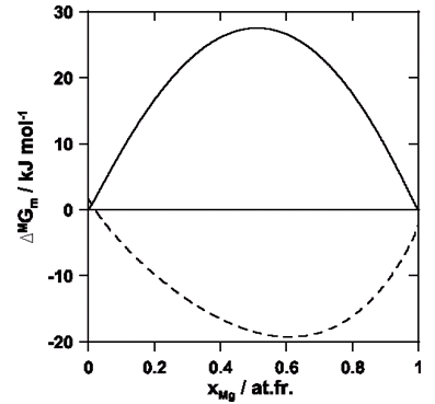
Figure 17: Calculated curves of Gibbs free-energy of mixing for Mg-Cu alloys at 1173 K (this work). —: crystalline phase, - - -: liquid phase. Reference: the mixture of the crystalline pure metals at 1173 K.

Table 5: Calculated (this work) and experimental values [37] of lattice parameters.

Conclusions
We have presented a MC calculation for the structural and thermodynamic study of Mg-Cu alloy. The calculation can reproduce a solid, a glass and a liquid structure when the phase diagram shows these structures as we can see with the resulting g(r) function (each case is analysed in the previous text). We have calculated the liquid with potentials fitted to the solid state. Lukens and Wagner [12] measurements of the radial distribution function and the existence of liquid order were confirmed. The calculations of Gibbs free energy, activities and heat of mixing for liquid at 1100 K were performed and the differences between experimental and calculated values in this work are much smaller than those presented by other authors [35]. Our simulation calculation was able to reproduce a point of the phase diagram.
The system with 256 atoms is enough to reproduce experimental results and the bigger cells do not show differences to be taken into account.
This is a first modelling calculation for Mg-Cu alloy using MC and we are able to confirm theoretically the previous experimental observations. Results improved considerably with respect to previous calculations with other techniques. We may therefore conclude that MC calculations are worth using in these studies. Also a potential fixed to solid state properties gave good results even for liquid structures. In the future it is desirable to have similar MC studies for other systems with available experimental data.

Acknowledgements:
The authors are grateful to Dr. Alicia Batana for her critical reading of the manuscript. They also acknowledge Dr. N. L. Allan for the MC program and fruitful discussions and Dr. E. O. Timmermann for his useful comments on thermodynamics aspects.

References

[1] Coughanow, C.A; Ansara, I.; Luoma, R.; Hämäläinen, M.; Lukas, H. L., Z. Metallkde. 1991, 82, 574.         [ Links ]

[2] Agrawal, R. D.; Mathur, V. N. S; Japoor, M. L., Trans. Jpn. Inst. Met 1979, 20, 323.         [ Links ]

[3] Sommer, F.; Lee, J. J.; Predel, B., Ber. Bunsenges. Phys. Chem, 1983, 87, 792.         [ Links ]

[4] de Boer F. R.; Boom R.; Mattens W. C. M.; Miedema A. R.; Niessen A.K., Cohesion in Metals., North-Holland, Amsterdam, 1988        [ Links ]

[5] de Tendler, R. H.; Kovacs, J.; Alonso, A; J. Mater. Sci., 1992, 27, 4935.         [ Links ]

[6] Bailey, .P.; Schiøtz, J.; Jacobsen, K. W.; Phys. Rev. 2004, B69, 144205        [ Links ]

[7] Bailey, .P.; Schiøtz, J; Jacobsen, K. W., Materials Science and Engineering A, 2004, 387, 996.         [ Links ]

[8] Daw, M. S.; Foiles, S. M.; Baskes, M. I., Matter. Sci. Rep. 1993, 9, 251.         [ Links ]

[9] Foiles, S. M, Phys. Rev., 1985, B 32, 3409.         [ Links ]

[10] Hultgren, R.; Desai, P. D.;Hawkins, S.; Gleiser, M.; Kelley, K.; Wagman, D., Selected Values of the Thermodynamic Properties of the Elements, (ASM, Metals Park, Ohio, 1973, Cu and Mg evaluation dated 1969).         [ Links ]

[11] Juneja, J. M., Iyengar G. N. K.; Abraham K. P., J. Chem.Thermodynamics, 1986, 18, 1025.         [ Links ]

[12] Lukens, W. E.; Wagner, C. N. J., Z. Naturforsch., 1973, 28 a, 297.         [ Links ]

[13] Sommer, F.; Bucher, G.; Predel, B., J.Phys. Colloque, 1980, C-8 41, 563.         [ Links ]

[14] Nayeb-Hashemi, A.A.; Clark, J. B., BAPD, 1984, 5, 536.         [ Links ]

[15] Kempen, A. T. W.; Nitsche, H.; Sommer, F.; Mittemeijer, E. J., Metallurgical and Materials Transactions, 2002, 33 A, 1041.         [ Links ]

[16] Marquez, F. M.; Cienfuegos, C.; Pongsai, B.K.; Lavrentiev, M. Yu; Allan, N. L., .Purton, J. A.; Barrera, G. D., Modelling Simul. Mater. Sci. Eng., 2002,10, 1.         [ Links ]

[17] Daw, M. S.; Baskes M. I, Phys. Rev., 1984, B 29, 6443.         [ Links ]

[18] Finnis, M. W.; Sinclair, J. E., Phil Mag 1984, A 50, 45.         [ Links ]

[19] Escolessi, F; Parrinello, M.; Dosatti, E., Phil Mag, 1988, 58, 213.         [ Links ]

[20] Kittel, C, Introduction to Solid State Physics, Wiley, New York, 6th ed., 1986.         [ Links ]

[21] Overton, W. C.; Gaffney, J, Phys. Rev., 1955, 98, 969.         [ Links ]

[22] Simmons, G.; Wang, H, Single Crystal Elastic Constants and Calculated Aggregate Properties: A Handbook, Massachusetts Institute of Technology, Cambridge, MA., 1971.         [ Links ]

[23] Eremenko, V. N.; Lukashenko, G. M.; Polotskaya, R I., Russ Metall, 1968,1, 126.         [ Links ]

[24] Barrera, G. D.; de Tendler, R, Comp. Phys. Commun., 1997, 105 159.         [ Links ]

[25] Metropolis, N.I.; Rosenblunth, A. W.; Rosenblunth, M. N.; Teller, A. H.; Teller, E. J., J. Chem. Phys., 1953, 21, 1087.         [ Links ]

[26] Purton, J.A.; Barrera, G.D.; Allan, N. L.; Blundy, J. D., J. Phys. Chem. B, 1998,102, 5202.         [ Links ]

[27] Frenkel, D.; Smit, B.; Understanding Molecular Simulation, Academic Press; San Diego, 1996.         [ Links ]

[28] Lavrentiev, M. Yu; Allan, N.L.; Barrera, G.D.; Purton, J.A., J. Phys. Chem. B, 2001, 105, 3594.         [ Links ]

[29] Touloukian, Y. S.; Kirby, R. K.; Tylor, R.E; Desai, P. D., Thermal Expansion; Metallic Elements and Alloys, IFI/Plenum, New York, 1975.         [ Links ]

[30] King, H.W.;“Crystal Structure of the Elements at 25 C”, Bull. Alloy Phase Diagrams, 2(3), 401-402, 1981.         [ Links ]

[31] JANAF Thermochemical Tables, 3rd ed. ed. by Davies, C.A.; Downey, J. R.; Frurip, D. J.; McDonald, R.A.; Syverud, A. N., J.Phys.Chem.Ref.Data , 1985, 14, Suppl. 1.         [ Links ]

[32] Waseda, Y., The Structure of Non-Crystalline Materials: Liquids and Amorphous Solids, McGraw-Hill, New York, 1980.         [ Links ]

[33] Table 2.1 in The Physical Properties of Liquid Metals by Takamichi, I. Guthrie, R. I. L, Clarendon Press, Oxford, 1993.         [ Links ]

[34] Koester, L, Neutron physics, Springer Tracts in modern Physics, 1977, 80,1.         [ Links ]

[35] Asta, M; Morgan, D.; Hoyt, J.J.; Sadigh, B.; Alhoff, J. D.; de Fontaine, Foiles, S. M., Physical Review, 1999, B59, 14271.         [ Links ]

[36] Turnbull, D., J.Appl.Physics ,1950, 21, 1022.         [ Links ]

[37] Bagnoud, P.; Feschotte, F., Z. Metallkde., 1978, 69, 114.         [ Links ]