Introduction

Structural analysis to determine the variability of a parameter field is a basic and essential step to be performed in geostatistical estimation or simulation of a parameter. Variographic analysis provides lot of information about the nature of the variable. This is performed in two steps viz., calculation of an experimental cova-riance/variogram and its modeling with theoretical one. The practical formula for calculating the experimental variogram needs translation of expected value to an arithmetic mean (Ahmed, 1995). This implies having sufficient number of pairs for each lag and the conventional procedure of calculating variogram does not have any control over the number of pairs. The present work provides a new approach for determination of experimental variograms with the desired number of pairs for each lag, which comprises an efficient and entirely new way of calculating variograms by keeping a control over the number of pairs.

Related Prior ArtIt is known from the Theory of Regionalized Variables that the various magnitudes, which are the function of time and space, are highly variable. However, these parameters are highly correlated among themselves. There exists some correlation between these variables when distributed in space or time. ^{Matheron (1965}, 1970, 1971) have termed these variables as the regionalized variables and claimed that they posses definite structure depending on the spatial correlation, at different locations. Mathematically the Regionalized variable is simply a function F(x) which takes a particular value at every point ‘x’ of the three-dimensional co-ordinate system. Generally a regionalized variable at any point x has an expected value, which we term as the mean. To estimate these regionalized variables, both stationary and non-statio-nary, the method of kriging was adopted. In certain cases, especially in hydrology, the hypothesis of second order stationarity with finite variance is not satisfied by the data. We assume that the variance is simply a function of the difference of locations of the data points and that the mean is constant. These assumptions comprise the intrinsic hypothesis. According to Marsily (1986) this variance of the increment gives the definition of the variogram. These variogram models controls the kriging weights assigned to the data points during the applications of kriging like interpolations, point estimation, block estimation, contouring, mapping, estimation of mean value. All the interpolation, estimation and contouring methods are based on the spatial correlation of data points. Thus Variography is the ‘heart’ of any geostatistical study. Experimental variograms plot the average difference of pairs (variance) of the data points against the distances (lag) separating these pairs. This plot of variance against lag fitted with a model curve is the “true variogram”. An experimental variogram is usually an irregular curve due to large value of lag and tolerance. Three parameters sill, range and nugget effect are the essential components to model the va-riogram curve. Marsily (1986), obtained the usual kriging equations based on the intrinsic hypothesis or in the second-order stationarity when the mean is unknown. In 1984, in a book, Dowd suggested some alternative methods for a robust and resistant variogram and found that localized drift has a significant effect on va-riogram estimation and these should be taken into account. In the same book M. ^{Armstrong (1984}), suggested the improvements in estimating and modeling the variogram. In yet another book by Isaak and Srivastava (1989) have discussed the concept of variogram calculation in details by graphically showing the idea of tolerance on distance lag with several examples. In the two papers by Zekai (1989, 1992), has shown the advantages of working on cumulative and standard cumulative variogram to introduce greater smoothness in experimental va-riogram but one has to derive a corresponding theoretical variogram.

De Smedt et al. (1985) have discussed about a variogram calculated from erroneous data and suggested that the true variogram could be obtained by removing the entire nugget effect. However, ^{Ahmed and Marsily (1987}), have clarified that the nugget effect is a combined result of small-scale variability and the erroneous data and since we do not know the variance of the data error, we simply cannot remove it. The nugget effect could be calibrated through cross-validation test. Cressie (1985), has described weighted least squares fit for a robust variogram estimator based on square root differences.

Journel and Hujbregts (1978), suggested that the number of data pairs in each class should be at least 30 and this rule of thumb seems to be widely accepted in the literature. Marsily (1986), propounded that the total number of pairs that can be formed from a set of ‘n’ points is n (n-1)/2. However, they are not evenly distributed. There are more pairs at short than at long distances (lag). Thus he cleared that at large distances the variogram becomes more uncertain. In personal communication Mathe-ron suggested that the minimum numbers of 30 pairs are required to fit a model variogram.

Variogram estimation is a crucial stage of spatial prediction, because it determines the kriging weights. It is important to have a variogram estimator, which remains close to the true underlying variogram, even if outliers (faulty observations) are present in data. Genton (1998), claimed that the classical variogram estimator proposed by Matheron is not robust against outliers in the data nor is it enough to make simple modifications such as the ones proposed by Cressie and Hawkins (1980), in order to achieve robustness. He reduces the percentage of outliers and then showed that robust estimation of variogram is better than the Matheron’s and Cressie’s. Cressie (1985) have tried to formalize the method of variogram fitting by setting out three possible approaches, Least squares, weighted least squares, in which the weighting is directly proportional to the number of observations and is larger for smaller lags. And third approach used by him is generalized least squares. He concluded that the weighted least square is the true compromise between simplicitly and statistical efficiency. A fit based on robust estimator needs less compromise than the Matheron estimator.

^{David (1977}) mention about weighting each variogram estimator according to the number of points involved in estimation, though he did not mention the method to adopt this technique.

^{Beckers and Bogaiert (1998}) have investigated the problem of estimating the variogram or covariance function when the mean of the random function is not stationary. They have used the residuals to estimate the variogram and have proposed a methodology to yield the accurate estimations of the variogram. It was an extension of the weighted Least Square method by Cressie (1985), Russo (1984), ^{Warrick and Myers (1987}), are among those who have proposed algorithms for designing spatial samples when the primary objective is reliable estimation of g by g1. A user of Russo’s procedure starts by specifying the number of lag classes and number of pairs of points to be included in each class, and the algorithm then produces a design for which the variation of lag values within each class is at least locally minimized. Warrick and Myers’ approach involves specifying the lag intervals to be employed and the desired number of pairs of points in each distance class, but their algorithm allows for classification of data pairs by angle to test the assumption of isotropy.

Morris (1991), stated that for planning the spatial sampling studies for the purpose of estimating the semivariogram, the number of data pairs separated by a given distance is sometimes used as a comparative index of the precision, which can be expected from a given sampling design.

All the works mentioned above have adopted the calculation of classical variograms, applicable to the dense data points. But in the case of hydrology we face the lack of dense datasets. We usually have the sparse data points and the sparse data sets. So there is a need for some estimation technique, which may be helpful and may prove worthy of estimating the data sets even in the presence of sparse data values. This new invention proclaimed by us proves to be worthy in case of sparse data sets and culminate the drawback of the lack of sufficient data set for estimation purposes.

Yet another aspect of approaching through this classical way of calculating the vario-grams is that the variograms calculated through this method has no control over the number of pairs to be taken into consideration. For calculating the variogram through the above-mentioned works, one has to decide the initial lag, tolerance, number of lags etc then only we can calculate simple or cross-variograms. The total number of pairs to be formed is calculated. There is complete freedom to the user to change the lag and tolerance in order to get the best fit of the model. There is no fixed rule to decide the lag to be given as an input. Therefore in this way the present invention is useful for keeping a control over the number of pairs to be computed. Since there is no hard and fast rule to choose the value of lag in the classical approach of calculating variogram, our method of determining the experimental variograms with ensured number of pairs for each lag proves to be an efficient and better approach for the sparse data sets.

In yet another embodiment of the present invention is that we get the proper fitting of the theoretical variogram, which was not possible in proceeding through the classical approach. While approaching through the traditional methods we get limited number of pairs or rather less number of pairs in case of sparse data sets. So the fitting of theoretical variogram over these limited pairs leads to erroneous model fit. Thus this new approach of generating the variograms comprises a robust and efficient process for the determination of Experimental Variograms with desired number of pairs for each lag and leads to a much better fit of theoretical variogram.

Still another advantage is that we are calculating the experimental variograms by considering all the constraints required for a variogram.

We have adopted a new approach of keeping a check over the number of pairs formed. Since the lag and tolerance are variable quantities and can be chosen according to the experimenter. There is no hard and fast rule to fix the initial lag and tolerance and therefore the numbers of pairs formed are different. This leads to the misleading or erroneous calculation of the variograms, thereby deteriorating the quality of the estimated parameters. But in the present approach we have the control over the number of pairs, which leads to a much better experimental variograms.

Program for calculation of variogramThe stepwise implementation of the algorithm is shown in below a flowchart, mentioned below:

• Reading of the data in X, Y, Z format where (X, Y) specifies the location of the data parameter and Z is the parameter on which the variographic analysis needs to be done.

• Calculation of the distance (D) between the respective location used the coordinates

Figure 1: Comparison between variogram of the water level data of srikakulam district. / Figura 1. Comparación entre variograma de los datos del nivel de agua del distrito de sri-kakulam. 

• In the first case we divide the total number of pairs equally after averaging them. If initial number of pairs obtained is Nd then in order to get final Ndf we choose (Nd / Ndf ) pairs to get the final values. Now we plot the values of averaged distance against the squared difference values in order to get the variogram plot.

• As the second case, we divide the total number of pairs Nd into randomly by giving the arbitrary value to number of pairs to be averaged. In this approach we get the output depending upon the initial number of pairs Nd formed.

• An important aspect of calculating the variograms through this process is that we keep the complete control over the necessary conditions and the constraints applicable to the definition of the variogram, as defined by the earlier workers.

A key factor that is fostering these calculations is the use of Excel and spreadsheet analysis. We have embraced and accepted the use of Excel to perform these above-mentioned calculations. It has been customary to use the spreadsheets for the analyses of hydrological datasets especially for the pumping test data and for the analysis of ground water problems. We have accepted the applicability of Excel for calculating these experimental variograms with the new approach of obtaining the ensured number of pairs. All the calculations performed can be easily implemented.

Figure 2: Flowchart for the calculation of variograms for the sparse datasets./ Figura 2. Diagrama de flujos para el calco de variogramas para conjuntos de datos dispersos. 

Figure 3: Calculated variograms for the resistivity data at site S1. / Figura 3. Variogramas calculados para los datos de resistividad en el sitio S1. 

Use of Excel support plotting of experimental variogram soon after the computation is done. For modeling the variogram, the accepted expression for theoretical variogram are supplied (Marsily, 1986) and theoretical variogram are supplied for matching.

Figure 1 shows the comparison between the variogram calculated on the same datasets but with different approaches. The two methods employed are

1. The conventional approach

2. The variograms calculated from the invented program in EXCEL

Variographic analyses of point resistivity dataOn the basis of the flowchart (figure 2) mentioned, the variograms for each acquired dataset of resistivity were calculated.

Figure 4: Comparative decrease in nugget effect. / Figura 4. Disminución comparativa en efecto pepita. 

We proceeded by first calculating the va-riogram at the respective location of resistivity data and then calculating the squared difference of the resistivity value at that particular location. In total there are 342 data points of resistivity in a 2D pseudosection of ERT programmed to obtain the data along the profile at S1 and S2 (data courtesy Arora and Ahmed, 2010). This leads to the formation of 58311 pairs. These pairs were arranged in the ascending order and their average was taken in different fashion. After doing a lot of exercise we found that the variogram with the average of 2000 pairs is the best to be modeled and provides the most relevant information.

The following figure 3 shows the different sets of calculated variogram for the resistivity obtained at S1. The first plotted value signifies the average of the initial 2000 pairs, and thus the corresponding ones. By calculating the variograms by this method we have a better control over the number of pairs. This is very much essential while dealing with the sparse datasets in hydrological society.

These variograms (figure 3) corresponds to the data acquired on the respective date as mentioned in the inset of the figure. These correspond to the resistivity data for the site S1.

Thus from the variographic analysis it may be noticed that there exist a decreasing pattern for the nugget effect as a whole including total sill value. In total there is 30 % at site S1 the nugget effect decreases to 30% and there is decrease in the variance percentage also, at S1 the variance decreases by 67 %. The decreasing trend is shown in figure 4.

Figure 5: Comparison of the variograms and the nugget effect at S1. / Figura 5. Comparasion de los variogramas y el efecto pepita en el S1. 

Figure 6: Calculated variograms for the resistivity data at site S2. / Figura 6. Variogramas calculados para los datos de resistividad en el sitio S2. 

Also this decrease is clear from the calculated variograms after comparing the initial and the final calculations as shown in figure 5 below.

Equivalent observation can be observed on another site S2, the decrease in resistivity is well correlated with the decrease in the nugget effect. The comparison is clear from figure 6 showing the variograms of resistivity at another site S2. These variograms (figure 6) corresponds to the data acquired on the respective date as mentioned in the inset of the figure. These correspond to the resistivity data for the site S2.

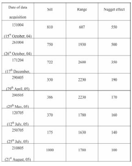
Table 1: Table showing the variogram parameters. / Tabla 1. Tabla mostrando los parametros de los variogramas. 

Thus from the variographic analysis it may be noticed that there exist a decreasing pattern for the nugget effect as a whole. At site S2 the nugget effect decreases to 60% once we move from pre monsoon to post monsoon. There is a decrease in the variance percentage also, at S2 by 78 %.

The decrease in nugget effect as well as total sill indicates the increase in correlation and continuity. In the pre monsoon condition, the moisture are scattered due to lesser availability of the medium. Soon after the rainfall event, soil moisture deficit is filled either partially or completely, the continuity increases as well as the saturation. Resistivity of the zone decreases overall but at the same time the variability also decreases and result in decrease of total sill as well as the nugget effect. By analyzing carefully around at a close interzone, we may also determine the time lag in the rainfall and recharge events.

Estimation of resistivity at points of mosture measurementsAs explained in the previous chapters the measurements of soil moisture and the point resistivity were taken at different supports due to obvious reasons of methodology and field setup. Also due to logistic reasons the time of measurements could not coincide but efforts were made to take measurements as close as possible. Geostatistical techniques of estimation were used to perform estimation of point resistivity values at points of moisture measurement.

The methodology of Block kriging was implemented to krige the soil electrical resistivity data at the locations where soil moisture were measured. Variograms for the ERT datasets were calculated and fitted with the theoretical variogram model, shown in table 1 below.

The parameters values and the variability were employed to krige the ERT data set at site S1. The soil moisture data was acquired at the interval of every 0.3 m. Neutron probe provide measurements of soil moisture at a value surrounding the measurement point i.e. 0.3 m in the present case. Thus block estimation of ERT data were made with a support of 0.3 m block.

Soil moisture (saturation) and electrical resistivity relationAfter kriging the resistivity data set at the collocated measurement points of soil moisture, the relationship between the two parameters was attempted. The above relationship exist between the saturated medium, thus this is the first attempt in the unsaturated media. As existing in the literature the relationship says that for initial 10 percent of soil moisture the resistivity shows a decreasing trend, later on after 15 percent even if the saturation increases there is no change in the resistivity values. Our results are shown below, figure 7.

The same sample from the field was investigated in the laboratory also to find the relation between electrical resistivity as an effect of desaturation of the sample, shown in figure 8 (Krishnamurthy personal communication, 2002). Soil samples from different depths were taken and analysed for determining their resistivity and saturation simultaneously using an electric oven in the laboratory. The samples were fully saturated initially and then it was dried up. During this process of drying up resistivity measurements were made using electrodes. A relation between the saturation and soil moisture resistivity were thus plotted by averaging the

Relation Between Resistivity and Soil Moisture (Field Data) results from different depths and in general a similar relation is formed (figure 7).

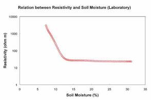
Figure 7: Relationship between the resistivity and soil moisture form the field data at S1. / Figura 7. Relación entre la resistividad y la humedad del suelo de los datos de campo en S1. 

These relations on one hand confirm the facts similarly both in field and laboratory conditions and also restrict the application of resistivity measurement to estimate soil moisture or recharge. However, the constant nature of resistivity arrives only after a fixed saturation say 15 % and since in the field conditions due to intermittent rainfall, the moisture often do not cross the limit and therefore, the technique is successfully applied in the field.

The following points should be pondered over

• Although the total sill indicates the high variability of the formation parameter but reduction in the nugget effect signals the increase in the continuity of moisture present that was more random before the rainfall. Prior to recharge there is no continuity of moisture, but after the rainfall there exists the continuity.

• Presence of nugget effect shows that the distribution of moisture, as observed with the resistivity and moisture profiles, is not continuous with depth. There exists some gaps and moisture exists in patches.

• But after the rainfall and the infiltration the gaps are filled and the distribution of the moisture becomes continuous.

• Graphical relation is established both in laboratory as well as in field that initially a non-linear relation exist between soil moisture and resistivity. However, the resistivity becomes invariant even with the moisture increase in the range of 11 % to 13 %.

Conclusion

Variography in calculating and modeling the va-riogram is an essential part of the geostatistical estimation. Calculation of experimental vario-gram from the measured field values is subjected to a number of approximations at various stages arising from the theoretical assumptions as well as field limitations like absence of measuring points on regular grids or in clustered fashion etc. Unlike other fields, most of the parameters in groundwater hydrology are measured from the wells and the wells are planned keeping entirely different aspects in mind. The calculation of variogram needs paired values at different but well distributed intervals and use of statistical approach further needs their number as large as possible. The most common approach of calculating the variogram proceeds by pre selecting a distance lag (interval) and a suitably allowed tolerance. There is normally no relation in the selection of lags and the locations of the measurement points and hence in case of sparse data that is often the case with hydrologic and hydrogeological parameters, very few numbers of pairs are obtained particularly for the smaller lags. That makes the variogram unreliable and changing lags randomly becomes much more time consuming and without assured result.

A new procedure has been developed to arrange all the possible pairs in ascending order and then picking up a desired number of pairs to calculate the experimental variogram by averaging the squared difference of their respective values. This procedure however, allows at one hand a complete freedom of taking any number of pairs one desires to overcome the limitations on the less number of pairs and make the variogram statistically reliable but on the other hand care has to be taken to obtain the resulting lag and inherent tolerance within the specified constraints. Thus calculations of mean and standard deviation of all the used intervals are made before finalizing the variogram and verify the constraints on lag and tolerance. If the conditions are not satisfied, the selection of pairs is changed and the procedure is revised. Obtaining an adequate selection of pairs with desired number is much simpler than changing the lags in classical approach. Another freedom is possible in this approach that the desired number of pairs could be kept either uniform for all the variograms or be varied. The uniform number of pairs for all the variograms favors and reduces the conditions on fitting a theoretical model. Using this approach, for the integration of the both different datasets, helps in obtaining the conclusive results. It further proves beneficial for the amalgamation of two different datasets and to bring them at a widespread stage. The variography process introduced here will be highly beneficial to the water scientists for optimizing their network, in the absence of enough datasets.

Figure 8: Relationship between the resistivity and soil moisture form the field data analyzed in the laboratory, at S1. / Figura 8. Relación entre la resistividad y humedad del suelo de los datos de campo analizados en el laboratorio, en S1. 

Acknowledgement

The author is grateful to Director, CSIR-NGRI for giving permission to publish this work. This study was funded by CSIR, India towards the doctoral thesis of the author and few figures are reproduced from it. The Editors and Reviewers are acknowledged for their continuous support towards improving this manuscript.