Economic sensor for Misiones Province from 2005 to 2018

(*) Nicolás Álvarez; (**) Juan Luis Heredia; (***) María Natalia León

(*) Facultad de Ciencias Económicas
Universidad Nacional de Misiones
Posadas, Misiones, Argentina
nalvarez@fce.unam.edu.ar

(**) Facultad de Ciencias Económicas
 Universidad Nacional de Misiones
Posadas, Misiones, Argentina
juanluish012@gmail.com

(***) Facultad de Ciencias Económicas
 Universidad Nacional de Misiones
Posadas, Misiones, Argentina
nleon@campus.unam.edu.ar

Reception Date: 06/03/2019- Approval Date: 06/19/2019

ABSTRACT

This paper presents the construction of a composite indicator of economic activity for the province of Misiones for the period 2005 – 2018, in order to measure fluctuations of economic and growth cycles. The methodologies proposed by The Conference Board (2001) and Jorrat (2003), that are referents at international and national levels respectively, are used. This methodology gives less weight to time series which variations have more volatility. After selecting eleven component series from public sources of information and representatives from different sectors of the provincial economic activity, seasonally adjusted using X-13 ARIMA and aggregating them, it is obtained a composite indicator representative for the economic activity, named Misiones Economic Sensor (MisES).
This indicator is a first approximation of provincial economic activity’s fluctuations, and given that cross correlation with EMAE (Mensual Estimator of Economic Activity) is 0.93 when t=0, it is presumed that it is represents fluctuations observed in the provincial economy.

KEY WORDS: Composite Index, Economic Activity, Regional Economy.

INTRODUCTION

Argentina is a country of great extension, only the Continental American surface has some 2,791,810 km2, considering the Continental Antarctic surface the value amounts to 3,761,274 km2 (Argentina, National Geographic Institute, 2019). It is the second largest country in Latin America and, at the same time, is the second largest economy after Brazil. This duality is not coincidence since the Argentine economy has benefited from the great wealth and variety of natural resources that it has throughout the land. The Argentine National Constitution, with the objective of economic and social development, contemplates the creation of regions, so that the provinces can make use of the natural resources existing in their territory (Article 124). The concept of region is carried out by establishing a division criteria that delimits the space according to the objective of the study, facilitating its better understanding (Valenzuela, 2007). However, the so-called productive regions are based on a criteria determined mainly by ecological factors, like average annual temperatures and rainfalls, although social and structural factors are possible as well, these factors configure what it can be called as ecoregions. Thus, in line with the INDEC regions, the following regions are taken into account: Northwest (NOA), Northeast (NEA), Cuyo, Pampeana and Patagónica. The natural production conditions of each ecoregion (climate, soil, relief, availability and quality of water) determine the heterogeneity of provincial economic activities (Ferraris, 2015). The province of Misiones is part of the NEA region, along with the provinces of Corrientes, Chaco and Formosa.
It is of great importance to have updated information on the evolution of economic activity so as to elaborate good quality public policies, and planning of production on the private sector. For this reason, at national level, the National Institute of Statistic and Census (INDEC), “Public organization of technical character, dependent of the Ministry of Treasury, which has faculties over official statistical activities that take place in the territory of the Republic of Argentina” (Argentina. Instituto Nacional de Estadísticas y Censos, 2019), calculates Gross Domestic Product (GDP), an indicator of aggregate production par excellence. On one hand, it allows us to know the value of final goods and services produced in the economy for a certain period of time. Additionally, to meet the need for updated and timely information, it calculates the Monthly Estimator of Economic Activity (EMAE) which “is a provisional indicator of the evolution of GDP at current prices that will be published with delay of 50 to 60 days after the end of the reference month, according to the INDEC’s diffusion calendar” (Argentina. Instituto Nacional de Estadísticas y Censos, 2016, p. 4). On the other hand, the estimation of the level of activity in the Argentine provinces was traditionally carried out through the calculation of the Gross Geographical Product (PBG in spanish), a task delegated to the provincial statistics institutes. Currently, there is no province that has frequent updates of its data, since most of them are annual and there are delays in their publication, which means that they are not opportune for the formulation of public policies and decision making (Muñoz, Ortner, & Pereira, 2008).
The need to have updated and constant information on the evolution of the level of economic activity has led provinces to search for a substitute / supplement calculation of the PBG (which requires a lot of time and resources), the same way that at national level the calculation of the GDP is complemented with the publication of the EMAE. The provinces of Chaco and Formosa discontinued the calculation of the PBG, presenting alternatively the analysis of the evolution of their economic activity through the elaboration of a composite indicator. The province of Corrientes, however, performs the calculation of the PBG quarterly, although there’s usually a delay in its publication. In the province of Misiones, the Institute of Statistics and Census (IPEC) publishes annual data of the PBG, which are calculated by the General Directorate of Revenue (DGR). That is, in the province of Misiones there is no indicator of economic activity with frequency higher than a year and with opportune availability. Also, it has no indicator of provincial economic activity alternative to the PBG.
Considering the importance for the provinces of having updated information on economic activity to improve and expand public policies as well as being useful for planning by the private sector, the construction of a composite indicator of economic activity, such as it is the EMAE or different provincial indicators, will allow an approximate representation of the evolution of economic activity in the province of Misiones, showing information summarized in a single indicator.
The work is structured as follows. First, a theoretical framework is made referring to the measurement of economic activity and cycles, emphasizing the consideration of different calculation alternatives applied to regional economies. Second, the methodology applied in the construction of a composite indicator of economic activity for the province of Misiones is described. Third, the results obtained are shown, making a subsequent discussion of them. Finally, the conclusions, limitations and implications of the work are presented.

DEVELOPMENT

Theoretical Framework
Economic activity is defined as any process in which products, goods or services are generated and exchanged. That is to say, an economic activity can be considered to be any activity that allows the generation of wealth within a community, and it can occur through the extraction, transformation and distribution of natural resources or of some service; in all cases, the final goal is the satisfaction of human needs.
The economy resorted to three major currents of thought at the time of explaining the large differences in income, conditioned by the development of economic activities that exist between the different regions: geography, integration and institutions (Rodrik & Subramanian, 2003). The current of thought that focuses on geography, as a preponderant factor in the generation of large income differences, is the oldest and most recognized theory where climate and natural resources are the key determinants, which in turn affect other factors; but mainly they determine the economic activities that are developed in the different regions.
The present work focuses on the characteristic factors of a given region shaped by their natural production conditions (climate, soil, relief, availability and water quality), originating the concept of productive regions, according to which, the economic activities that are developed in a certain region are configuring what are called regional economies (Ferraris, 2015).
For the measurement of economic activity different indicators are used. One of the most used over time by different countries is the Gross Domestic Product (GDP). In general terms, it is composed of the aggregate values generated by the productive units resident in a given economic territory. However, when calculating the product of a jurisdiction that represents a portion of the country’s total territory (for example, a province), there are difficulties in determining the residence jurisdiction of the productive units that develop their activities in more than one jurisdiction. The calculation of the Gross Geographical Product has managed to overcome this difficulty.
The Gross Geographical Product (PBG in Spanish) as defined by Gropper for CEPAL (an organization that helped estimate and publish an annual update of provincial PBGs in Argentina) is "the calculation of the Product of a jurisdiction that represents a portion of the country’s total territory" (Gropper, nd, p. 3). That is, following the concept adopted by Gropper, "the Gross Domestic Product of a given jurisdiction should reflect the economic activity of the productive units resident in that jurisdiction" (Gropper, nd, p. 3). An important concept in this definition is the delimitation of the jurisdictions that represent the economic territory; in this case, they are given by the political borders of the provinces.
Both the GDP and the PBG demand a lot of resources and time for their elaboration due to the exhaustive calculation, so alternative indicators are taken into consideration. In this sense, composite indicators of economic activity emerge seeking to reflect the evolution of the level of economic activity based on the combination of several sectorial indicators. To elaborate them, there are several methodologies depending both on the statistical criterion used, as the criterion with which the variables are selected, and the weight given to them.
Burns & Mitchell (1946) developed a definition of economic cycles and based on it, they built a methodology of composite indicators of economic activity that currently is the main reference worldwide. Since its inception, the Economic Cycles Program of the National Bureau of Economic Research (NBER), the U.S. Department of Commerce Bureau of Economic Analysis and more recently The Conference Board, have relied on this indicator approach. In Argentina, one of the pioneers in the construction of composite indicators of economic activity is Juan Mario Jorrat who prepared the Monthly Index of Economic Activity of Tucumán (IMAT) and the Coincident Composite Index of Argentina (ICCO). The ICCO is the first antecedent of a composite indicator of economic activity at national level and  is elaborated on the basis of coincident series and has a monthly periodicity, having a correlation both in levels and in logarithmic variations with respect to GDP of 0.98 and 0.80 respectively (Jorrat, 2003; Jorrat, 2005).
At national level, the INDEC calculates the Monthly Estimator of Economic Activity (EMAE) developed by the National Institute of Statistics and Censuses (INDEC), which measures the activity of different sectors of the Argentine economy by means of indicators that are representative of each one, in order to combine them and generate an indicator that can be useful to measure the variations of the national GDP (INDEC, 2016). As for the measurement of the economic activity for a jurisdiction that represents a portion of the national territory, Jorrat (2003), develops a methodology that is used for the construction of the Monthly Index of Economic Activity of Tucumán (IMAT), seasonally adjusted series using the program X-12-ARIMA and determine the turning points using the Bry & Boschan procedure. Contrary to this, Muñoz & Trombetta (2008) developed a synthetic indicator of economic activity for the 24 provinces and for the Argentine Republic using the methodology of The Conference Board (2001) with modifications that do not change the spirit of the algorithm. Both the IMAT and the ISAP use updated statistical information of public access with monthly or quarterly frequency. Michel Rivero (2007) developed an indicator of monthly economic activity for the province of Córdoba (ICA-COR), analyzing the economic activity of the province from 1994 to 2006. In addition, D'Jorge, Cohan, Henderson, & Sagua (2007) created the ICASFe, a coincident monthly activity index for Santa Fe. Both the ICA-COR and the ICASFe, used the methodology proposed by Jorrat in the construction of the IMAT. Lapelle (2013), following the traditional methodology of The Conference Board, developed a synthetic indicator of coincident economic activity for the Rosario region (ISARR) considering the period from 1993 to 2011.
The concept of economic cycles adheres to the notion that aggregate economic activity does not show constant growth and, in turn, experiences occasional shocks of activity and recession. Burns & Mitchell (1946:3) define business cycles (also known as economic cycles) as:

Business cycles are a type of fluctuation found in the aggregate economic activity of nations (...)  a cycle consists of expansions occurring at about the same time in many economic activities, followed by similarly general recessions, contractions, and revivals which merge into the expansion phase of the next cycle; this sequence of changes is recurrent but not periodic; in duration business cycles vary from more than one year to ten or twelve years; they are not divisible into shorter cycles of similar character with amplitudes approximating their own (Burns & Mitchell, 1946, p. 3).

What is implicit in the definition of Burns & Mitchell (1946), and the methodology of the NBER, is the assumption that there is an unobserved variable common to all sectors, which they call Economic Cycles. This latent variable can be approximated or expressed by the average weight of a number of statistical indicators. This definition of business cycles has two relevant characteristics; the first is the existence of co-movement or common movements between the different economic variables; the second is the division of economic cycles into separate phases or regimes, dealing differently with expansions and recessions (Diebold & Rudebusch, 1996).
At national level, Jorrat (2005) proposes a way to establish recessions or expansions based on the determination of peaks or troughs of economic cycles. The peaks are the relative maximums of the economic activity, while the troughs are their relative minimums. The expansions would be between a trough and a peak; the opposite happens with recessions, defined between peaks and troughs. Therefore, both peaks and troughs are called turning points.
In contrast, growth cycles are characterized by fluctuations in economic activity around their trend. When economic activity is above its long-term trend, there is an acceleration of growth; whereas the deviations below their tendency are denominated deceleration of the growth (Jorrat, 2005).
It is very important to differentiate growth cycles from economic cycles since the former refers to fluctuations in economic activity with respect to the long-term trend, while the latter are the fluctuations that occur in the levels of economic activity.
The province of Misiones is the province with the highest population and economic activity in the NEA region. The climate and the properties of the land allowed an expansion of its primary sector, in addition to the natural attractions that arouse the tourist activity (IPEC, 2015). The PBG of the province of Misiones in 2005 represented 1.2% of the GDP at national level, a percentage that was already observed, and remained approximately constant, since 1997. While its participation at national level did not vary, its participation did within the NEA region which increased by almost one percentage point (29.1 % - 30%). Opposite to this, in the same period (1997-2005), the aggregate product of the region lost participation in the national total (4.1% - 3.8%) (Argentina. Ministry of Economy and Public Finance, 2013; Argentina. Ministry of Finance, 2017).
The economic activities that take place in the province of Misiones can be summarized in three main sectors: primary (11.40%); secondary (37.40%); and tertiary (51.20%) (Misiones. Instituto Provincial de Estadísticas y Censos, 2015). Regarding specific productive activities, the most relevant at provincial level, in physical production volume, are: yerba mate, cellulose pulp, tea and industrialized wood products (Argentina. Ministry of Finance, 2017).
The province has 16 border crossings with Brazil and another 13 with Paraguay, 90% of the provincial perimeter has international borders making commercial flow with neighboring countries relevant for local income, and many national macroeconomic variables affect in greater proportion to their productive and commercial activities (Freaza, 1993, Freaza & Ibarra, 2016, Misiones. Instituto Provincial de Estadísticas y Censos, 2015).

Methodology
For the construction of a composite indicator of monthly economic activity for the province of Misiones, considering references both at national and international level, it is necessary to carry out the following steps:
1. Determination of a reference indicator.
2. Selection of the component series.
3. Treatment of series.
4. Aggregation of series.
5. Contrast with the reference indicator.
6. Extraction of cycle.
7. Determination of turning points.

1. Determination of a reference indicator
Firstly, it is necessary to have a reference indicator of the economic activity of the region to be studied. This is relevant when establishing the representativeness of the constructed indicator, both of the fluctuations of the economic activity and of the cycles that it has. In Argentina, several indicators constructed for provinces have used GDP as a reference indicator (Jorrat, 2005, Michel Rivero, 2007, D'Jorge et al, 2007), since most of them do not have an indicator of their own activity with frequency higher than a year.
In the present work, by not having a provincial indicator of reference with the features of the composite indicator to be constructed, the EMAE is used as a reference, which reflects the variations in GDP with monthly frequency.
2. Selection of the component variables.
Regarding the selection of the component variables, the criteria adopted by The Conference Board (2001:14) are considered:

• Economic Significance, there must be an economic argument when selecting the variables.

• Statistical Adequacy, data must be collected and processed in a statistically reliable way.

• Consistent Timing, the series must show a synchronization pattern consisting of time as a leading indicator, coincident or lagged.

• Conformity, the series must adjust well to the economic cycle.

• Smoothness, its movement from one period to another cannot be very erratic.

• Availability or delay of the information, the series must be published reasonably quickly.

It is important to emphasize that the component series do not strictly comply with all of these requirements, however, these criteria are used with some flexibility. The main criteria to be taken into account in the present work are: economic significance, delay in the availability of information and compliance. Nevertheless, all the criteria are taken into account.
The Conference Board (2001) chooses four variables referred to the level of employment, personal income, industrial production and industrial sales. They were considered as reference dimensions when selecting economically significant component series for the province of Misiones. In addition, due to the importance of fiscal resources for the Argentine provinces, it was decided to consider a fiscal dimension.

Table N° 1. Dimensions, indicators and weights of component series of composite indicator of economic activity

Source: Own elaboration

(*) Monthly series. Exceptions are EMPD and IVA.
(**) Weight is the result of methodology of construction.

One of the main productive sectors of the province, the forestry sector, was not included as there were no variables that matched the selection criteria for this work. Misiones’s Ministry of Ecology conducts surveys related to the amount of wood outflow of the province, but said indicator doesn’t fill the required criteria and is countercyclical to the reference cycle, counteracting other variables effect.
3. Treatment of the series
In the case of the nominal series, it is necessary to carry out a deflation process, for which the Inflación Verdadera CPI is used (Cavallo & Bertolotto, 2016). Since it is available for almost the entire period of analysis from January 2005 to November 2018 to forecast the value of December 2018, it is chained with the CPI published by the INDEC. It is clarified that the nominal series are deflated at 2005 values.
Then, the series are seasonally adjusted using the X-13 ARIMA program, which adjusts the series by calendars, Easter, outliers and level changes effects. The X-13, through an iterative process, seasonally adjusts series and provides outputs which contain series adjusted by seasonality, trend-cycle and irregular. Out of these different tables, table E2, C17 and D12 will be used. Table E2 is the seasonally adjusted series (At) adjusted by irregulars, table C17 are the weights (Wt) which vary from 1 to 0 for outliers of the irregular component, and table D12 the Trend-Cycle component (Tt).
So the adjusted series used, following Jorrat (2003) will be:

If Wt = 0, the series at time t will be equal to the value of table D12 and E2; if Wt = 1, the value used for time t will be from table E2; in case 0 < Wt < 1, then the resulting value will be an average of table E2 and table D12 for time t. For more details on the process of seasonality treatment carried out by the X-13 program, see Jorrat (2003).
In order to aggregate quarterly series with monthly series, quarterly series are transformed into monthly series by applying cubic splines.

4. Aggregation of Series.
  The Conference Board (2001:47) proceeds with the following steps in order to aggregate selected variables:

1. Calculate monthly variations, r(i,t), for each component, x(i,t), where i = 1, …, n. For the components that are in percent form, the following difference has to be done: r(i,t) = x(i,t) – x(i,t)-1. In other cases, percent change formula is used: r(i,t) = 200 * (x(i,t) - x(i,t-1)) / (x(i,t) + x(i,t+1)).

2. Adjust month to month changes by multiplying them by the component’s standardization factor, wi. The monthly contributions for each component i are C(i,t) = wi * r(i,t). Wi It’s the inverse of the standard deviation of symmetric percent change of series which penalize components with greater volatility. Standardization factors are normalized so the summation can be equal to 1.

3. Add adjusted monthly changes. This is the summation of adjusted contributions St = ∑ n(i=1) C(i,t).

4. Calculate preliminary levels of the index using symmetric percentage change formula. Index is calculated recursively, starting with an initial value of 100 for the first month of the sample. Let I1 = 100 be the initial value of the index of the first month. If s2 is the result of step c) for the second month, preliminary value of the index is:

Then the value of the preliminary index for the following month is:

*Rebase index to average 100 in the base year. Preliminary levels of the index obtained in step d) are multiplied by 100 and divided by the mean of preliminary levels of the index in the base year.

5.  Contrast with the reference indicator.
  A cross correlation analysis between the reference indicator and the MisES is carried out with the purpose of knowing if the resulting indicator is coincident with the reference indicator.
6. Extraction of cycle.
For extracting the cycle component of the indicator to elaborate, the Hodrick-Prescott filter is used. Even though there is no generalized agreement of what λ value has to be used. λ = 14400 is considered, value recommended by Mazzi & Scocco (2003) for monthly series.
7. Determination of Turning Points
  The method employed to determine turning points is the Bry & Boschan algorithm, which are exhibited by Mazzi & Scocco (2003:19):

1. Peaks and troughs must alternate.

2. Each phase that is from peak to trough and from trough to peak must have a minimum duration of 6 months.

3. A cycle that is from peak to peak or trough to trough, must have a minimum duration of 15 months.

4. Turning points within six months of the beginning or end of the series are eliminated as are peaks or troughs within 24 months of the beginning or end of the series if any of the points after or before are higher (or lower) than the peak (trough).

Results
Once the necessary steps have been established, component series were selected, treating them by seasonality and other particular considerations, so as to be aggregated in order to obtain a composite indicator representative of the provincial economic activity.
First, a cross correlation analysis was carried out between component indicators and the reference series, EMAE, to validate them. It’s important to emphasize that the static series is the reference one.

Table N° 2. Correlation between EMAE and component series

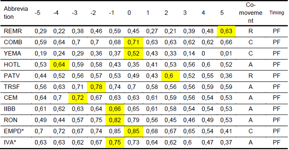
Source: Own Elaboration

(*) Quarterly series.

Ref.: A = leading; C = Coincident; R = Lagging; PF = Procyclical – strongly.
As can be seen in Table Nº 2, all the selected variables have a correlation greater than 0.5 (being positive all of them) in the maximum correlation with the EMAE, therefore they have pro-cyclical timing of strong intensity. There are two lagging indicators, PATV and REMR. Likewise, the maximum correlation of REMR is at time t = 5, a value that does not differ much from the moment t = -1, the same happens for the case of PATV where its maximum occurs at t = 2, a value that does not differ from the moment t = -2. These values ​​are due to the fact that seasonal or irregular movements are affecting the series, but after seasonality treatment their correlations are at their maximum when t = 0 being the only exception the YEMA series.
After the selection and subsequent treatment of the component series, they are aggregated to obtain the composite indicator of economic activity for the province of Misiones; it is named as Economic Sensor for the province of Misiones (MisES).
In MisES construction, series that have more weighting are (see Table Nº 1): Registered Employment in the Private Sector (0.3903); Real Remuneration in the Private Sector (0.1483); IVA levy (0.0865); Sale of Hydrocarbons (0.0824); Yerba Mate for Consumption (0.0659) and resources of national origin transferred to the province (0.0645).

Figure N° 1. Composite Indicator of Economic Activity for Misiones Province (MisES), from 2005 to 2018, 2005=100
Source: Own Elaboration

Due to its construction, the indicator can be interpreted as the level of activity that the province of Misiones has at a particular point in time. Figure No. 1 shows that since January 2005 (MisES = 100) until July 2017 (MisES = 183.74) the indicator has an increasing trend that, from August 2017, decreases until November 2018 (MisES = 146.72) at a value that was approximate in May 2011 (MisES = 146.04). The accumulated growth in the analysis period was 47.84%.
Cross correlation between EMAE and MisES is not only important in order to know if its correlation is high, but more importantly at what time it is high.

Table N°3. Cross correlation between MisES and EMAE

Source: Own Elaboration

Ref.: A = leading; C = Coincident; R = lagging; PF = Procycling – strongly.

At all t moments, the correlation is greater than 0.5 and positive, characterizing the indicator under study as strongly procyclical, reaching the maximum at t = 0; which would classify MisES as a coincident indicator of economic activity. That is, MisES is an indicator that has concurrent variations to the reference series.

Figure N° 2. Misiones Economic Sensor (MisES) y Monthy Estimator of Economic Activity (EMAE), 2005 – 2018 period, 2005=100
Source: Own Elaboration

The fact that the correlation is high when t=0 (MisES and EMAE), would indicate that the turning points should be at close moments in time, for both peaks and troughs. These will allow us to know in which periods there were recession and growth in the economy of the Province of Misiones.

Table N°4.  Comparative analysis of turning points of Business Cycle of MisES and EMAE

Source: Own Elaboration

In the first place, the number of turning points detected by the algorithm for the MisES is lower than those presented by the EMAE, having a correspondence of 78% (number of turning points detected for the MisES in relation to those of the EMAE). This may be due to the fact that the analysis corresponds to the economic cycle and not to the growth one, with the latter having a better performance in the detection of turning points (Jorrat, 2005). Second, the differences between the turning points dates of both indicators are relatively low, with an average of -0.14, which would classify the indicator as coincident with the EMAE (Jorrat, 2005), reinforcing the results of the cross correlation (Table Nº 3).

The evidence provided by the composite indicator demonstrates that the economic activity of the province of Misiones goes into recession a period of time after recession started at national level, this is true for all turning points except for 2017.09 (September 2017), almost the same happens with the troughs, where the only exception is for 2009.05 (May 2009) where the date is the same for both indicators.

Figure N° 3. Deviation of MisES from its long term trend, from 2005 to 2018
Source: Own Elaboration

Table N°5. Comparative analysis of turning points of MisES and EMAE growth cycles

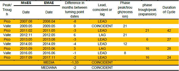
Source: Own Elaboration

First, there’s a 100% correspondence in the quantity of turning points dated between the growth cycle of the EMAE and the MisES. However, the difference in months between one date and another is between -8 and 6, with the average of the difference in months of the turning points -1.33, characterizing once again the indicator as a coincident one. The dates of the turning points of the economic cycles are different from those of growth, since the latter precedes the former. In the case of peaks of growth (starting point of a slowdown), these occur before or simultaneously to the peaks of economic cycles (starting point of a recession) since there is a slowdown in the growth of the economy at the beginning, and then the recession occurs. The opposite can be said about troughs of growth.

Discussion of Research Outcomes
The resulting indicator fulfilled the objectives of the present work. However, it is only a first approximation to the behavior of the provincial economic activity. The lack of a reference indicator for the Province of Misiones does not allow us to evaluate to what extent the result is representative of itself.  For its construction, it was encountered the lack of other available indicators due to the inexistence of many of them, for being temporarily short to be included, low frequency observations (e.g. yearly observations) or there being restricted access to data.
As can be seen, the resulting indicator under study differs from the levels of the reference indicator (EMAE) and this is due to several reasons. First, the EMAE measures the national economic activity, adding observations up to the national level; while the MisES adds observations up to the provincial level. Second, they differ in their component indicators. Third, aggregation and calculation methodologies are different in both indicators. For all these reasons, indicators have different interpretations (EMAE refers to the level of national economic activity, whereas MisES to the level of provincial economic activity) but this is no obstacle from comparing them with each other. Also, there are different methodologies to adjust the levels of an indicator to the reference. Muñoz et al (2008) try to find a set of weights for each component that minimizes the sum of the square differences between the EMAE and the ISAP levels, obtaining as a result a synthetic indicator of economic activity with approximate levels to the EMAE. In contrast, Jorrat (2003), in the process of aggregation of the variables, adjusts the sum of the variations by amplitude and trend of the reference indicator, in this case the GDP.
For the purpose of this research, it was decided not to make an adjustment to any reference indicator in order to exhibit the fluctuations of the provincial economy, and show how the variations of the component indicators affect MisES. Nevertheless, as can be seen in the correlation analysis the resulting indicator for the provincial economy shows a behavior very similar to that of the reference indicator. In this case, the maximum cross correlation is when t = 0 which led to the conclusion that the variations between the MisES and the EMAE are similar concurrently, something that would be confirming the close relationship between the provincial economic activity and the national. Other indicators that use the EMAE as a reference, such as the ISARR or the ISAP, resulted to be coincident indicators of economic activity (Lapelle, 2013, Muñoz et al, 2008). On the contrary, the Leading Index for Argentina, developed by Jorrat (2005), is an indicator that provides early information on changes in the turning points for the Argentine economy. If a similar indicator were developed for Misiones, it would be necessary to find a set of variables and/or a specific methodology that can anticipate changes in the phases of provincial economic activity.

CONCLUSION

In the present work a composite indicator of economic activity for the province of Misiones was created, named Misiones Economic Sensor (MisES) with monthly periodicity, having a correlation of 0.93 (t = 0) with the Monthly Estimator of Economic Activity (EMAE) published by the INDEC. Therefore, it is a coincident indicator of economic activity compared to the variable reference with fluctuations similar to those presented in the national economy, so its behavior is presumed to be representative of the provincial economic activity.
Regarding the analysis of economic cycles, it was observed a pattern in which MisES apparently tends to enter recession some time later than national economic activity. On the opposite side, the economic activity of the province recovers sooner than national economic activity. All of this means that recessive phase of the provincial economic cycle are shorter than the expansive phase in contrast to EMAE’s behavior.
The similarity between MisES and EMAE, an indicator that measures the national economic activity, led to consider the importance of the sectors that are relevant to the province of Misiones which could not be represented by a pertinent indicator, particularly the external sector through the real exchange rate, and those related to forestry-industrial production. In respect of the first issue, it is recognized that the Province of Misiones has borders with Paraguay and Brazil and as mentioned by Freaza (1993), the exchange differences are important, affecting the commerce of tradable goods, and in the particular case of Misiones the non-tradable. Any change in the real exchange rate at a certain level can affect the regions involved positively and negatively. Therefore, it is important to conduct a more in-depth study on how to construct and include that variable in the activity indicator. In regard to the second issue, it is not unknown the importance of the wood industry of Misiones, the reason being the absolute advantages that its geography presents for forestry development, and the companies that produce cellulose pulp that are present in the region. Therefore, it is left for future research a study to determine how it would impact obtaining and incorporating an indicator representative of that sector when doing an approximation of the provincial economic activity’s behavior. The production of sectorial statistics will not only allow knowing the situation of a certain sector or activity, something that in itself would represent an improvement, it would allow to measure with greater fidelity the aggregate economic activity of the province of Misiones.
This work is considered to be a first approximation to results of a research that will continue to be developed in search of improvements related to different methodologies and the incorporation of new indicators not available to date. Thanks to the projections provided by the X-13-ARIMA, the indicator can be updated to the reference month; technique that will be subject of post-analysis of the value estimated with respect to the observed value. Regarding relevant indicators to be incorporated, those related to the external and forestry sector of the province of Misiones should be subject of research.

NOTES

In Jorrat the process of seasonality adjustment of X-12 is explained. The only difference between the X-13 is that the latter incorporates a second option (SEATS method) for seasonality treatment.

Percentage change formula treats positive and negative changes symmetrically. When a 1 percentage increase followed by a 1 percentage decrease occurs, the level of the index returns to its initial value. This is not true when conventional formula 100 * (Xt - Xt-1)/Xt-1, is used, because same percentage changes would underestimate the actual value of X (The Conference Board, 2019).

REFERENCES

Please refer to articles in Spanish Bibliography.

BIBLIOGRAPHICAL ABSTRACT

Please refer to articles Spanish Biographical abstract.

1.Argentina. Instituto Geográfico Nacional. (30 de Mayo de 2019). Límites, superficies y puntos extremos. Obtenido de Instituto Geográfico Nacional: https://www.ign.gob.ar/NuestrasActividades/Geografia/DatosArgentina/LimitesSuperficiesyPuntosExtremos
2.         [ Links ]Argentina. Instituto Nacional de Estadística y Censos. (2016). Metodología del Estimador Mensual de la Actividad Económica, EMAE. Ciudad Autónoma de Buenos Aires: Instituto Nacional de Estadística y Censos. Recuperado el 3 de Julio de 2017, de https://www.indec.gov.ar/ftp/cuadros/economia/metodologia_emae_ago_16.pdf
3.         [ Links ]Argentina. Instituto Nacional de Estadísticas y Censos. (5 de Junio de 2019). El INDEC. Obtenido de INDEC: https://www.indec.gob.ar/el-indec.asp
4.         [ Links ]Argentina. Ministerio de Economía y Finanzas Públicas. (2013). Provincia de Misiones. Buenos Aires: Ministerio de Economía y Finanzas Públicas.         [ Links ]
5.Argentina. Ministerio de Hacienda. (29 de Noviembre de 2017). Actividades productivas relevantes por provincia: Misiones. Obtenido de Información económica provincial y municipal: https://www2.mecon.gov.ar/hacienda/dinrep/mapas/datosPorProvincia.php?provincia=misiones
6.         [ Links ]Burns, A. F., & Mitchell, W. C. (1946). Measuring business cycles. Boston: National Bureau of Economic Research. Obtenido de https://papers.nber.org/books/burn46-1
7.         [ Links ]Cavallo, A., & Bertolotto, M. (2016). Cambridge: The Billion Prices Project. Recuperado el 30 de mayo de 2019, de https://www.thebillionpricesproject.com/wp-content/papers/FillingTheGap.pdf
8.         [ Links ]D´Jorge, M. L., Cohan, P. P., Henderson, S. J., & Sagua, C. E. (2007). Proceso de construcción del Índice Compuesto Coincidente Mensual de Actividad Económica de la provincia de Santa Fe (ICASFe). Centro de Estudios y Servicios de la Bolsa de Comercio de Santa Fe. Ciudad de Buenos Aires: Asociación Argentina de Economía Política. Recuperado el 3 de Julio de 2017, de https://www.aaep.org.ar/anales/works/works2007/d_jorge%20.pdf
9.         [ Links ]Diebold, F. X., & Rudebusch, G. D. (27 de Junio de 1996). Measuring business cycles: a modern perspective. Review of Economics and Statistics, 78(1), 67-77. Obtenido de https://www.nber.org/papers/w4643.pdf
10.         [ Links ]Ferraris, G. (2015). Introducción al estudio de las Regiones Productivas de la Argentina. En F. d. Forestales, Regiones Productivas de la Argentina (págs. 2-13). La Plata: Universidad Nacional de La Plata. Recuperado el 30 de Mayo de 2019, de https://www.ing.unlp.edu.ar/catedras/G0433/descargar.php?secc=0&id=G0433&id_inc=21751
11.         [ Links ]Freaza, M. A. (1993). La economía de Misiones y su inserción en el contexto regional. Posadas: EdUNaM - Editorial Universitaria de la Universidad Nacional de Misiones.         [ Links ]
12.Freaza, M. A., & Ibarra, Z. N. (2016). Indicadores económicos de la provincia de Misiones: período 2002 - 2012. Posadas, Misiones, Argentina: EdUNaM - Editorial Universitaria de la Universidad Nacional de Misiones.         [ Links ]
13.García-Carro Peña, B., & Cancelo de la Torre, J. R. (2000). Un sistema de indicadores cíclicos para la economía gallega. Oviedo, Principado de Asturias, España: ASEPELT España. Recuperado el 3 de Julio de 2017, de https://www.asepelt.org/ficheros/File/Anales/2000%20-%20Oviedo/Trabajos/PDF/250.pdf
14.         [ Links ]Gropper, D. (s/f). Propuesta metodológica para el cálculo del Producto Bruto Geográfico en Argentina. Buenos Aires: CEPAL.         [ Links ]
15.Jorrat, J. M. (2003). Indicador Económico Regional: El Índice Mensual de Actividad Económica de Tucumán (IMAT). Universidad Nacional de Tucumán. Ciudad de Buenos Aires: Asociación Argentina de Economía Política. Recuperado el 3 de Julio de 2017, de https://aaep.org.ar/anales/works/works2003/Jorrat.pdf
16.         [ Links ]Jorrat, J. M. (2005). Construcción de indices compuestos mensuales coincidente y líder de Argentina. En M. Marchionni (ed.), Progresos en econometría (págs. 43-100). Buenos Aires: Asociación Argentina de Economía Política.         [ Links ]
17.Lapelle, H. C. (2013). El Indicador Sintético de Actividad para la Región Rosario (ISARR) 1993-2012. Ciudad de Buenos Aires: Asociación Argentina de Economía Política (AAEP). Recuperado el 3 de Julio de 2017, de https://aaep.org.ar/anales/works/works2013/lapelle.pdf
18.         [ Links ]Mazzi, G. L., & Ozyildirim, A. (2013). Business cycles theories: an historical overview. En U. Nations, Handbook on cyclical composite indicators (Draft) (págs. 23-62). Nueva York: United Nations.         [ Links ]
19.Mazzi, G. L., & Scocco, M. (2003). Bussiness cycles analysis and related software applications. Luxemburgo: Office for Official Publications of the Europeans Communities. Recuperado el 26 de agosto de 2017, de https://ec.europa.eu/eurostat/documents/3888793/5815721/KS-AN-03-013-EN.PDF
20.         [ Links ]Michel Rivero, A. D. (2007). (U. N. Instituto de Economía y Finanzas (IEF), Ed.) Revista de Economía y Estadística, 45(1), 31-73. Recuperado el 3 de Julio de 2017, de file:///G:/Descargas/3835-17165-1-PB.pdf
21.         [ Links ]Misiones. Instituto Provincial de Estadísticas y Censos. (2015). Gran atlas de Misiones. Posadas, Misiones, Argentina: Instituto Provincial de Estadística y Censos. Recuperado el 20 de Junio de 2017, de https://www.ipecmisiones.org/gran-atlas-de-misiones
22.         [ Links ]Muñoz, F., & Trombetta, M. (2014). Indicador Sintético de Actividad Provincial (ISAP): un aporte al análisis de las economías regionales. Varias. Ciudad de Buenos Aires: Asociación Argentina de Economía Política. Recuperado el 3 de Julio de 2017, de https://aaep.org.ar/anales/works/works2014/munoz.pdf
23.         [ Links ]Muñoz, F., Ortner, J., & Pereira, M. (2008). Indicador Sintético de Actividad de las Provincias (ISAP): un aporte al análisis de las economías. Buenos Aires: Asociación Argentina de Economía Política. Recuperado el 30 de Mayo de 2019, de https://aaep.org.ar/anales/works/works2008/munoz.pdf
24.         [ Links ]Rodrik, D., & Subramanian, A. (Junio de 2003). La primacía de las instituciones (y lo que implica). Finanzas & Desarrollo, 31-34.         [ Links ]
25.The Conference Board. (2001). Business cycle indicators handbook. New York, United States of America: The Conference Board. Recuperado el 3 de Julio de 2017, de https://www.conference-board.org/pdf_free/economics/bci/BCI-Handbook.pdf
26.The Conference Board. (30 de Mayo de 2019). Calculating the Composite Indexes. Obtenido de The Conference Board: https://www.conference-board.org/data/bci/index.cfm?id=2154
27.Valenzuela, C. (2007). Abordajes recientes en torno a la investigación de las Economías Regionales. El caso del Nordeste Argentino. En O. Graciano, S. Lázzaro, & (comp.), La Argentina rural del siglo XX. Fuentes, problemas y métodos (págs. 185-212). Buenos Aires: La Colmena.         [ Links ]