Servicios Personalizados
Revista
Articulo
Indicadores
-
 Citado por SciELO
Links relacionados
-
 Similares en
SciELO
  uBio
uBio
Compartir
Phyton (Buenos Aires)
versión On-line ISSN 1851-5657
Phyton (B. Aires) vol.79 no.1 Vicente López ene./jun. 2010
ARTÍCULOS ORIGINALES
Statistical models for evaluating the genotype-environment interaction in maize (Zea mays L.)
Modelos estadísticos para evaluar la interacción genotipo-ambiente en maíz (Zea mays L.)
Kandus1 M, D Almorza3, R Boggio Ronceros2, JC Salerno1
1 Instituto de Genética, IGEAF, INTA, Castelar, Buenos Aires, Argentina.
2 Facultad de Agronomía, UNCPBA, Buenos Aires, Argentina.
3 Universidad de Cádiz, España.
Address Correspondence to: Ing. Agr. M. Sc. Mariana Virginia Kandus, e-mail: mkandus@cnia.inta.gov.ar
Recibido - Received 20.I.2010.
Aceptado - Accepted 25.II.2010.
Abstract. Our objective was to determine the genotype-environment interaction (GxE) in a hybrid integrated by maize lines either carrying or not balanced lethal systems. Experiments were conducted in three locations over a period of two years considering each year-location combination as a different environment. Yield data were analysed using the Additive Main Effects and Multiplicative Interaction (AMMI) model and the Sites Regression Analysis (SREG). Results were represented by biplots. The AMMI analysis was the best model for determining the interaction.
Keywords: Adaptability; Multivariate analysis; Plant breeding; Stability.
Resumen. Nuestro objetivo fue determinar la interacción genotipo-ambiente (GxA) en híbridos integrados por líneas de maíz con y sin sistemas de letales balanceados. Los experimentos se condujeron en tres sitios durante dos años. Se consideró cada combinación año-sitio como un ambiente diferente. Los datos de rendimiento fueron analizados utilizando el modelo de interacción multiplicativo (AMMI) y de efectos principales aditivo, y el análisis de regresión de los sitios (SREG). Los resultados fueron representados utilizando gráficos biplot. El análisis AMMI fue el mejor modelo para determinar la interacción GxA.
Palabras clave: Adaptabilidad; Análisis Multivariado; Mejoramiento vegetal; Estabilidad.
INTRODUCTION
Factors that are of economic relevance may be related to complex or poligenic characteristics, and show a high influence of the environment. Because of this, in breeding programs, various experiments are conducted in several locations to evaluate grain yield. In these experiments, changes in the relative behaviour of the genotype in different environments are usually observed. This phenomenon is called genotype by environment interaction (GxE), and it is the rule in most quantitative characteristics (Bernardo, 2002). The GxE interaction makes it difficult to select genotypes that produce high yields and that are more stable in breeding programs. This, of course, reduces the selection progress (Yan & Hunt, 1998).
The study of the GxE interaction allows the classification of genotypes by their behaviour in two different situations, either stable or adapted to a particular environment in terms of their yield or in some other interesting agronomic feature. Generally, the term stability refers to the ability of the genotypes to be consistent, both with high or low yield levels in various environments. On the other hand, adaptability refers to the adjustment of an organism to its environment, e.g., a genotype that produces high yields in specific environmental conditions and poor yields in another environment (Balzarini et al., 2005).
There are many statistical methods available to analyse the GxE interaction: for example, combined ANOVA, stability analysis and multivariate methods.
Combined ANOVA is more often used to identify the existence of GxE interactions in multi-environmental experiments. However, the main limitation of this analysis is the assumption of homogeneity of variance among environments required to determine genotype differences. Although this analysis allows the determination of the components of variance arising from different factors (genotype, environment and the GxE interaction), it does not allow to explore the response of the genotypes in the non-additive term: the GxE interaction (Zobel et al., 1998; Gauch, 1992).
Stability analysis provides a general solution for the response of the genotypes to environmental change. In this way, Yates and Cochran (1938) proposed linear regression analysis, which has been widely used and revised by a number of authors (Finlay & Wilkinson, 1963; Eberhart & Russell, 1966; Lin & Thompson, 1975; Becker & León, 1988; Crossa, 1990). This analysis, which involves regressing the average of the genotypes on an environmental index (the average yield of all the genotypes evaluated in each environment), provides a stability index. However, the analysis has several limitations and criticisms from both the biological and statistical points of view. The main biological problem appears when only a few very low and very high yielding sites are included in the analysis, and the fit is determined by the genotype behaviour in a few extreme environments (Crossa, 1990). The main statistical problem is that the average of all genotypes evaluated in each environment is not independent of the average of each genotype in a particular environment (Freeman & Perkins, 1971). Another statistical limitation is that the errors associated with the slopes of the genotypes are not statistically independent. The last problem is the assumption of a linear relationship between interaction and environmental means, when the actual responses of the genotypes to the environments are intrinsically multivariated (Crossa et al., 1990).
Multivariate analysis has three main purposes: (i) to eliminate "noise" in the data set (for example, to distinguish systematic and non-systematic variation); (ii) to summarize the information and (iii) to reveal a structure in the data (Crossa et al., 1990; Gauch, 1992). Models based on principal components analysis, such as AMMI and SREG, are linear-bilinear models with an additive component (the main effect of the environment or genotypes) and a multiplicative component (the GxE interaction).
AMMI is a combination of ANOVA for the main effects of the genotypes and the environment together with principal components analysis (ACP) of the genotype-environment interaction (Zobel et al., 1998; Gauch, 1988). AMMI models are usually called AMMI(1), AMMI(2), ..., AMMI(n), depending on the number of principal components used to study the interaction. Graphic representations are obtained using biplots (Gabriel, 1971) that allow (1) the observation, in the same graph, of the genotypes (points) and the environments (vectors), and (2) the exploration of patterns attributable to the effects of GxE interaction. In the biplot, the angles between the vectors that represent genotypes and environments show the interaction, and the distances from the origin indicate the degree of interaction that the genotypes show throughout the environments or vice versa.
Site regression analysis, SREG (Cornelius et al., 1996; Crossa & Cornelius, 1997; Crossa et al., 2002), also called GGE (Genotype Main Effect plus Genotype-Environment Interaction), is a linear-bilinear model that removes the effect of location and expresses the answer only as a function of the effect of genotypes and the GxE interaction. This model is recommended when the environments are the main source of variation in relation to the contributions of the genotypes and the GxE interaction with respect to the total variability (Balzarini et al., 2005). In addition, as a difference with AMMI model, this technique allows the detection of GxE interactions in terms of the crossover effect resulting from great changes in the ranking of the genotypes across the environments (Yan et al., 2000). Yan et al. (2000) used GGE biplot graphics to visualize patterns and interactions without environmental effects. These authors point out that usually the first principal component (CP1) represents responses of the genotypes that are proportional to the environments, which are associated with the GxE interaction without change of the range. The second principal component (CP2) provides information about cultivation locations that are not proportional to the environments, indicating that those are responsible of the GxE crossover interaction. At the same time, this technique allows the determination of mega-environments, which mean parts of the cultivation area of a species that show homogeneous environmental conditions, where the performance of certain genotypes is similar through the years (Gauch & Zobel, 1997). In each mega-environment, the effects of the genotype-location interaction are limited or negligible (Yan & Hunt, 2002).
The goal of this study was to evaluate the GxE interaction using AMMI and SREG for the yield of maize lines either with or without balanced lethal systems (BLS), and hybrids obtained after crossing all of these lines.
MATERIALS AND METHODS
Materials. Six BLS lines of flint maize from the Genetic Institute of INTA Castelar (BLS61, BLS91, BLS1, BLS101, BLS16 and BLS14), two different "Normal" lines (without BLS) from the INTA Pergamino (LP109 and LP521) and a commercial hybrid (ACA 2000) as a control, were used.
Methods. Self polinization and controlled crosses by hand were made among the eight inbreed lines over two years. All possible combinations were obtained, resulting in 28 hybrids (15 "BLS-BLS"; 12 "BLS-Normal" and 1 "Normal-Normal"). Then, grain yield of the hybrids and the parental lines were assessed in field trials, including the ACA 2000 hybrid that was considered "Normal-Normal".
The experiments were conducted in three locations: Castelar (34° 36' 48" S - 58° 39' 32" W), La Plata (34° 52' S - 57° 58' W) and Azul (36° 48' S - 59° 51' W), during two years under dryland conditions except in "Castelar Riego" which received irrigation (Table 1). The design used in all locations was a randomized complete block design with two replications. At harvest, grain yield per plot was measured, and the data were expressed as kg/ha.
Table 1. Code used in the biplot analyses for each location and year.
Tabla 1. Códigos usados en el análisis de dos ejes para cada lugar y año.
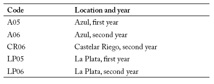
The genotype-environment interaction was evaluated with the AMMI model by considering the first two principal components. First, an ANOVA model was used to the yield data with main effects of genotype and environment (without the interaction), then, a principal component analysis (ACP) was fitted using the standardized residuals. These residuals include the experimental error and the effect of the GxE interaction. The equation was:
where Yij is the observed mean yield of the ith genotype in the jth environment,
μ is the general mean,
Gi and Ej represent the effects of the genotype and environment, respectively,
λk is the singular value of the kth axis in the principal component analysis,
αik is the eigenvector of the ith genotype for the kth axis,
γjk is the eigenvector of the jth environment for the kth axis,
n is the number of principal components in the model, and
eij is the average of the corresponding random errors.
An AMMI biplot representation was obtained, to explore only the pattern produced by the GxE interaction.
The following SREG model was also fitted. The equation was:
where Yij is the observed mean yield of the ith genotype in the jth environment,
__ Yi is the mean of the genotypes in the jth environment,
λ1 and λ2 are the eigenvalues for the two principal components, CP1 and CP2,
ξi1 and ξj2 are the scores for the ith genotype on components CP1 and CP2,
ηi1 and ηj2 are the scores for the jth environment on components CP1 and CP2, and
εij is the residual term associated with the average of the ith genotype in the jth environment centred by the effect of the jth environment.
A GGE biplot was obtained to explore patterns produced by the GxE interaction, to discover which genotypes obtained the highest and the lowest yields in each environment and to distinguish mega-environments. To determine a mega-environment in a graphical form, the extreme genotypes of the biplot were joined to form a polygon, and then perpendicular lines were drawn on each side of the polygon through the origin.
AMMI and SREG models, including biplot graphics and discrimination of mega-environments were obtained automatically with Infogen Professional Software (v. 2007).
RESULTS
Lines. Two first principal components (CP) of the AMMI model explained 82% of the data variability. The angle between the genotype and environment vectors determined the nature of the interaction; that is, it was positive for acute angles, negligible for right angles, and negative for obtuse angles. At the same time, the angle formed by the vectors of two environments provided an estimate of their correlation. In this way, the environments "La Plata first year (LP05)" and "Azul second year (A06)" were similar in their discrimination of the genotypes, being highly correlated and associated with positive values of CP1. At the same time, the environments "La Plata second year (LP06)" and "Castelar Riego second year (CR06)" were completely opposite in their discrimination of the genotypes, being associated with negative values of CP1. "Azul first year (A05)" was not correlated with the others, and explained the variability of the data in terms of CP2.
Orthogonal projections of the genotypes on the environmental vector showed that line BLS101 was better adapted to environments LP05 and A06, while lines LP109 and BLS91 were more stable as they were located near the origin. Line BLS61 was poorly adapted to environment A05. Lines LP521 and BLS16 were better adapted to LP06. Line BLS1 was better adapted to CR06 while line BLS14 had a good performance in both environments (Fig. 1).
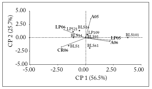
Fig. 1. AMMI biplot for "BLS" and "Normal" lines. Points represent lines and vectors represent environments.
Fig 1. Ejes AMMI par alas líneas "BLS" y "Normal". Los puntos representan líneas y los vectores representan ambientes.
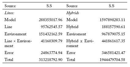
The sum of squares for the effect of the environment was greater than the sum of squares for the effect of the lines plus the GxE interaction, being 48.3% and 43.7% of the total sum of squares, respectively (Table 2), allowing data analysis with the SREG model. The first two principal components for this model explained 93% of the data variability. However, CP1 explained the largest percentage of the variability (76.5%). The environments LP05, A05, LP06 and A06 were more associated with CP1, while CR06 was more associated with CP2. At the same time, environments LP05, A05 and A06 were highly correlated among themselves and also with LP06, to a lesser level. However, they did not have any association with CR06. Of the five mega-environments that could be distinguished, only two included the environments LP05, A05 and A06 (mega-environment I), and the mega-environment II included CR06, while LP06 was on the boundary between these two mega-environments. Mega-environments IV and V were opposite to mega-environments I and II, respectively, so that the genotypes included in mega-environments IV and V were poorly adapted to mega-environments I and II, and vice versa.
Table 2. Sum of squares (SS) of the joint analysis of variance for yield of lines and hybrids in the considered environments.
Tabla 2. Suma de cuadrados (SS) para el análisis de varianza conjunto para el rendimiento de las líneas e híbridos en los ambientes considerados.
The relative yield from one genotype in a certain environment is the length of the environmental vector multiplied by the length of the orthogonal projection of each genotype on the vector. In this sense, CP1 separated BLS101 and BLS14 lines from the other lines, and they attained a greater yield in all the environments. In particular, BLS101 line was better adapted and obtained higher yields in environments LP05, A05 and A06 (mega-environment I). A similar trend occurred for BLS14 line in environments LP06 and CR6 (mega-environment II). Lines BLS61, BLS91 and BLS1 were more stable, and their yields were similar to the average of all the experiments. By contrast, lines LP109, LP521 and BLS16 showed a lower yield and were poorly adapted to mega-environment I (Fig. 2).
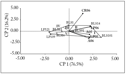
Fig. 2. GGE Biplot and discrimination of mega-environments (roman numbers) for "BLS" and "Normal" lines. Points represent lines and vectors represent environments.
Fig 2. Dos ejes para GGE y discriminación de grandes ambientes (números romanos) para "BLS" y "Normal". Los puntos representan líneas y los vectores representan ambientes.
Hybrids. The two first principal components explained 60% of the data variability using the AMMI model. From the biplot analysis, it was observed that CP1 separated the first of the second year, which were similar to those observed in the AMMI biplot obtained for the lines. The environments "La Plata first year (LP05)" and "Azul first year (A05)" were located on positive values of CP1. Meanwhile, "La Plata second year (LP06)", "Castelar Riego second year (CR06)" and "Azul second year (A06)" were completely opposite in their discrimination of the genotypes. At the same time, environments LP05 and LP06 were completely opposite to A05 and A06, respectively, as the angle formed by the vectors was 180°.
For positive values of CP1, the hybrids ACA2000 and LP109 x LP521 ("Normal-Normal") and BLS101 x BLS1, BLS61 x BLS16 and BLS16 x BLS14 ("BLS-BLS") were better adapted to A05. In addition, BLS61 x BLS101, BLS16 x BLS1 and BLS101 x BLS16 ("BLS-BLS") were better adapted to LP05 environment. On the other hand, the hybrids BLS14 x LP521, BLS61 x LP109 ("BLSNormal") and BLS101 x BLS14 ("BLS-BLS") were better adapted to A06. BLS61 x BLS91 and BLS14 x BLS1
("BLS-BLS") were better adapted to CR06, and the combinations BLS61 x BLS14 and BLS61 x BLS1 ("BLS-BLS") were better adapted to LP06. BLS91 x BLS1, BLS91 x BLS101 and BLS91 x BLS14 ("BLS-BLS"), and BLS91 x LP109, BLS16 x LP109, BLS61 x LP521, BLS1 x LP521 and BLS16 x LP521 ("BLS-Normal") showed a stable behaviour (Fig. 3).
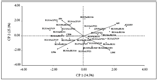
Fig. 3. AMMI biplot for the "Normal-Normal" (cursive font), "BLS-Normal" (normal font) and "BLS-BLS" (bold font) hybrids. Points represent hybrids and vectors represent environments.
Fig 3. Ejes para AMMI para los híbridos "Normal-Normal" (letra cursiva), "BLS-Normal" (letra normal) y "BLS-BLS" (letra en negrita). Los puntos representan a los híbridos y los vectores a los ambientes.
The sum of squares for the effects of the environment was greater than the sum of squares for the hybrids plus the GxE interaction, being 49.8% and 32.4% of the total sum of squares, respectively (Table 2). This allowed the evaluation of the data using SREG. The first two principal components for this model explained a low proportion of the data variability (53%). A05 and LP05 environments explained the variation at the CP1 level, and CR06 and LP06 explained the variation in CP2. From the biplot analysis, it was observed that the pairs of environment A05 - LP05 and A06 - LP06 were similar in their discrimination of the genotypes. Similarly to the GGE biplot obtained for the lines, the environment CR06 was different from the other environments.
Although five mega-environments were distinguished, only two of them included environments LP05, A06 and LP06 (mega-environment I) and the mega-environment II included A05 and CR06. Mega-environments III and IV were opposites of mega-environments I and II, respectively, so genotypes included in mega-environments III and (IV - V) were poorly adapted to mega-environments I and II, and vice versa. This implied the presence of crossover interactions among the genotypes included in these opposite mega-environments.
The right side of the biplot shows the higher yielding hybrids and vice-versa. Hybrids ACA2000 and LP109 x LP521 (highest yields), and BLS14 x BLS1 and BLS101 x LP109 (lowest yield), were the most extreme genotypes, and produced a greater contribution to the GxE interaction. In particular, genotypes BLS16 x LP521 and ACA2000 were better adapted to A05, while BLS1 x LP521 was better adapted to CR06 (mega-environment II). Hybrids LP109 x LP521 and BLS101 x BLS1 were better adapted to environments LP05 and A06 (mega-environment I) and, to a lesser extent, to A05. On the contrary, the hybrids with the poorest yield were BLS14 x BLS1 and BLS101 x LP521 (mega-environment III), and BLS101 x LP109, BLS61 x LP109 and BLS14 x LP109 (mega-environment IV). The combinations BLS16 x BLS1, BLS61 x BLS101, BLS61 x BLS14 and BLS91 x BLS14 (BSL-BLS), and BLS61 x LP521, BLS91 x LP521 and BLS16 x LP109 ("BLS-Normal") showed a yield similar to the average and had a more stable behaviour. Only BLS91 x BLS14, BLS16 x LP109 and BLS61 x LP521 hybrids were stable in AMMI and SREG models (Fig. 4).
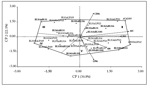
Fig. 4. GGE biplot and discrimination of mega-environments (roman numbers) for the "Normal-Normal" (cursive font), "BLS-Normal" (normal font) and "BLS-BLS" (bold font) hybrids. Points represent hybrids and vectors represent environments.
Fig 4. Ejes para GGE y discriminación de grandes ambientes (números romanos) para los híbridos "Normal-Normal" (letra cursiva), "BLS-Normal" (letra normal) y "BLS-BLS" (letra en negrita). Los puntos representan a los híbridos y los vectores a los ambientes.
DISCUSSION
1. The analysis of the GxE interaction was different in AMMI and SREG models. This occurred because the patterns obtained in the AMMI biplots allowed an exploration of the effects of the GxE interaction, while in the GGE biplot not only the interaction was observed but also the genotypes were superior in each environment.
2. Both models explained a high proportion of the data variability in the case of the lines. BLS61 and BLS91 lines were the most stable in terms of yield in both models. Line BLS101 provided the largest contribution to the observed interaction in both analyses, showing a specific adaptation to environments "La Plata first year" and"Azul second year", under AMMI model and to "La Plata first year", "Azul first year" and "Azul second year", under SREG model.
3. The lines BLS101 and BLS14 showed a high positive interaction in the environments in study, suggesting a greater specific adaptation than the other lines. On the contrary, lines LP109 and LP521 had a negative interaction with the environments in study, implying that they were poorly adapted. SREG showed that the lines BLS101 and BLS14 obtained a greater yield, opposite to LP109 and LP521.
4. AMMI model showed a better-defined pattern in the hybrids than did the SREG model for the relations among genotypes and environments, since the first principal component separated the effects of the first year from the second year. This pattern was not so evident in the lines. This finding was consistent with weather conditions, indicating that precipitation during January was greater in the first year than in the second year.
5. AMMI and SREG models explained a low percentage of the data variability. in the hybrid An unclear pattern was observed in relation to the type of hybrid ("BLS-BLS", "BLS-Normal" or "Normal-Normal"), and their behaviour in terms of stability or adaptability. AMMI and SREG models showed that the "BLS-BLS" and "BLS-Normal" hybrids had a more stable behaviour in terms of their yield. Among them, BLS91 x BLS14, BLS16 x LP109 and BLS61 x LP521 had a stable behaviour in both analyses. On the other hand, ACA2000 and LP109 x LP521 ("Normal-Normal" ), BLS101 x LP109 ("BLS-Normal") and BLS101 x BLS1 ("BLS-BLS") hybrids were among the genotypes that showed a specific adaptation to one or several environments that were correlated, which was consistent in both models.
6. The hybrids ACA2000, LP109 x LP521 and BLS101 x BLS1 had a positive interaction with the environments. This means that they were specifically adapted to most of the environments evaluated, and produced the highest levels of yield. The opposite trend occurred for BLS14 x BLS1 and BLS101 x LP109 hybrids. Both groups of hybrids were extreme genotypes in the SREG analysis, and contributed greatly to the GxE interaction. "BLS-BLS" hybrids, such as BLS91 x BLS16 and BLS61 x BLS91, were extreme genotypes at the CP2 level for the SREG model. This would indicate the existence of crossover interactions between them, mainly in "Castelar Riego second year" and "La Plata second year".
7. The SREG model allowed the visualization of high associations among locations without any relationship with the year of evaluation. These environments were different from the "Castelar Riego second year" in the lines as in the hybrids. This would indicate that La Plata and Azul are similar with respect to discrimination of the genotypes and that the effect of a high hydric availability (in Castelar) made the differences between environments larger than the differences in latitude. The results obtained for the differentiation of mega-environments did not agree exactly with those correlations among environments. This would indicate that the discrimination of mega-environments has a higher utility when there are a large number of locations with different environmental conditions, which reduce the number of experiments and, therefore, provides future cost savings. In this sense, Epinat-Le Signor et al. (2001) suggested that the evaluation of hybrids in representative conditions of the crop area is very important for identifying genotypes that are more stable and have larger yields. For this reason, to evaluate different BLS lines and their hybrids in future research, it is necessary to test different environments.
8. The results of this paper showed that the AMMI and SREG analyses allowed the identification of stable genotypes, and others that are better adapted to a particular environment. Several authors have used AMMI to evaluate multi-environment experiments of maize (Betrán et al., 2003; Gauch & Zobel, 1997), as well as SREG model (Fan et al., 2007). Gauch (2006) showed that AMMI analysis is better than SREG, because it allows to distinguish the effects of the genotype and the environment and then assess the GxE interaction in a reduced dimensional space with minimum error. Gauch & Zobel (1988) quantified the benefits of using AMMI that are equivalent to increase from two to five times the number of replications. For these reasons, AMMI would be the best model in multi-environmental experiments, and would provide an understanding of complex genotype-environment interactions (Gauch & Zobel, 1988; Zobel et al., 1988; Crossa et al., 1990; Gauch, 2006). However, SREG analysis has been widely used in breeding programs because it allows the visualization of the genotype grain yields in each environment. For this reason, the model selection will depend on the objective of the investigation.
REFERENCES
1. Balzarini, M., C. Bruno & A. Arroyo (2005). Análisis de ensayos agrícolas multi-ambientales: Ejemplos con Info-Gen. Fac. de Cs. Agropec. U.N.C., Argentina, 141 p. [ Links ]
2. Becker, H. C. & J. León (1988). Stability analysis in plant breeding. Plant Breeding 101: 1-23. [ Links ]
3. Bernardo, R. (2002). Genotype x environment interaction. In: Bernardo, R. (ed.) Breeding for quantitative traits in plants. Stemma Press. Woodbury, MN. pp 147-171. [ Links ]
4. Betrán, F.J., D. Beck, M. Bänziger & G.O. Edmeades (2003). Genetic analysis of inbred and hybrid grain yield under stress and nonstress environments in tropical maize. Crop Science 43: 807-817. [ Links ]
5. Cornelius, P.L., J. Crossa & M.S. Seyedsadr (1996). Statistical test and estimators of multiplicative models for genotype-by-environment interaction. In: Kang, M.S. and Gauch, H.G. (eds.). Genotype-byenvironment interaction. Boca Raton, FL, CRC Press. pp 199- 234. [ Links ]
6. Crossa, J. (1990). Statistical analysis of multilocation trials. Advances in Agronomy 44: 55-85. [ Links ]
7. Crossa, J., H.G. Gauch & R.W. Zobel (1990). Additive main effects and multiplicative interaction analysis of two international maize cultivar trials. Crop Science 30: 493-500. [ Links ]
8. Crossa, J. & P.L. Cornelius (1997). Sites regression and shifted multiplicative model clustering of cultivar trials sites under heterogeneity of variances. Crop Science 37: 406-415. [ Links ]
9. Crossa, J., P.L. Cornelius & W. Yan (2002). Biplots of linear-bilinear models for studying crossover genotype - environment interaction. Crop Science 42: 619-633. [ Links ]
10. Eberhart, S. A. & W.A. Russell (1966). Stability parameters for comparing varieties. Crop Science 6: 36-40. [ Links ]
11. Epinat-Le Signor, C., S. Dousse, J. Lorgeou, J.B. Denis, R. Bonhomme, P. Carolo & A. Charcosset (2001). Interpretation of genotype x environment interactions for early maize hybrids over 12 years. Crop Science 41: 663-669. [ Links ]
12. Fan, X.M., M.S. Kang, H. Chen, Y. Zhang, J. Tan & C. Xu (2007). Yield stability of maize hybrids evaluated in multi-environment trials in Yunnan, China. Agronomy Journal 99: 220-228. [ Links ]
13. Finlay, K.W. & G.N. Wilkinson (1963). The analysis of adaptation in a plant breeding programme. Australian Journal of Agricultural Research 14: 742-754. [ Links ]
14. Freeman, G.H. & J.M. Perkins (1971). Environmental and genotype-environmental components of variability. VIII. Relation between genotypes grown at different environments and measures of these environments. Heredity 27: 15-23. [ Links ]
15. Gabriel, K.R. (1971). Biplot display of multivariate matrices with application to principal components analysis. Biometrika 58: 453-467. [ Links ]
16. Gauch, H.G. Jr. (1988). Model selection and validation for yield trials with interaction. Biometrics 44: 705-715. [ Links ]
17. Gauch, H.G. & R.W. Zobel (1988). Predictive and postdictive success of statistical analyses of yield trials. Theoretical and Applied Genetics 76: 1-10. [ Links ]
18. Gauch, H.G. Jr. (1992). AMMI and related models. In: Gauch, H.G. (ed.) Statistical analysis of regional trials. Elsevier Science Publishers. The Netherlands. [ Links ]
19. Gauch, H.G. & R.W. Zobel (1997). Identifying mega-environments and targeting genotypes. Crop Science 37: 311-326. [ Links ]
20. Gauch, H.G. Jr. (2006). Statistical analysis of yield trials by AMMI and GGE. Crop Science 46: 1488-1500. [ Links ]
21. Lin, C.S. & B. Thompson (1975). An empirical method of grouping genotypes based on a linear function of the genotype-environment interaction. Heredity 34: 255-263. [ Links ]
22. Yan, W. & L.A. Hunt (1998). Genotype by environment interaction and crop yield. Plant Breeding Reviews 16: 135-178. [ Links ]
23. Yan, W., L.A. Hunt, Q. Sheng & Z. Szlavnics (2000). Cultivar evaluation and mega-environment investigation based on the GGE biplot. Crop Science 40: 597-605. [ Links ]
24. Yan, W. & L.A. Hunt (2002). Biplot analysis of diallel data. Crop Science 42: 21-30. [ Links ]
25. Yates, F. & W.G. Cochran (1938). The analysis of groups of experiments. Journal of Agricultural Science 28: 556-580. [ Links ]
26. Zobel, R.W., M.J. Wright & H.G. Gauch (1988). Statistical analysis of a yield trial. Agronomy Journal 80: 388-393. [ Links ]


