Introduction

The assessment of the impact of discharges on watercourses, such assewage or industrial ones, is essential for the sustainable management of water resources and the preservation of their quality. For this reason, it is necessary to know the evolution of the concentrations of incoming pollutants and of the resource's own compounds, axially and longitudinally, and their dependence on mixing parameters, kinetics of chemical reactions and flow models.

Accordingly, dispersion plays an important role in the transport of pollutants in water resources. When a pollution source, which has a density close to the density of water, is injected into the river, it propagates through the river and is transmitted downstream due to molecular motion, flow turbulence and shear dispersion. One of the main parameters discussed in river water quality problems is the dispersion coefficients, whether they are one-, two- or three-dimensional [1, 2].

In general, the mixing of pollutants is governed by the Advection - Dispersion (ADE) processes [^{3, 4, 5}]. In shallow rivers, the transverse velocity gradient rules the mixing process [6]; therefore, the equation of the ADE model can be written as (Eq. 1)

where C is concentration; t is time, x is distance from the source (i.e. the distance from when a certain pollutant or substance enters the river to the point where its concentration is determined), D _L is the longitudinal dispersion coefficient and U is the flow velocity.

As it can be seen in Eq. 1, D _L represents the pollution rate and is mainly used in water pollution modelling studies. Therefore, knowing the longitudinal dispersion mechanism in natural channels is of vital importance to control water pollution [7].

For the calculation of D _L , not only empirical established equations as a function of hydraulic parameters but also conservative tracer tests have been widely used.

Some of the current equations in literature are those of Liu [8], Fischer et al [3], Thomann and Mueller [9], Iwasa and Aya [10], Seo and Cheong [¹¹] and Kousis et al [12]. However, such equations display great variability in their results [13] as they were estimated for certain flow characteristics and are highly influenced by the presence of vegetation, meandering, channel geometry and slope, etc.

Several authors have been working on improving this type of prediction equations by decreasing the uncertainty [14, 15, 16, 17]. Fischer et al [3] presents an integral equation (Eq. 2) that takes into account particular characteristics of the flow since it allows D _L to be obtained through a detailed hydrodynamic characterisation of the section.

Where A is the cross-sectional area, u’(y) is the difference between the longitudinal average velocity in the verticalin the transverse progressive d the overall average velocity in h(y) depth in the progressive y; and dispersion coefficient in the progressive y.

Eq. 2 is based on the concept of uniform flow in a constant cross-section and as a counterpart, this equation requires a large amount of velocity and bathymetry information across the width of the section, which is not often available. On the other hand, it involves the calculation of ε _t , whose value is also subject to some uncertainty.

Despite the availability of such equations, in the D _L determination at an specific section of study in a river, conservative tracer tests are still the most accurate method [18].

When a non-conservative substance enters a body of water, it is physically transported through the advection and dispersion phenomena and may be subject to various chemical and biological reactions as well as phase transfer. No matter what type of water body it is, lakes, reservoirs, rivers, estuaries or oceans, they can be considered as various reactors in which constituents start to be transported or transformed. Mathematical models originally developed for chemical engineering can be translated into the description of the fate of these constituents in an aquatic environment [19]. A river can be modelled by applying the same design procedure of non-ideal chemical reactors, starting from tracer concentration data versus time (Curve C) in a certain section of the reach under study.

Therefore, statistical parameters such as the average residence time t(Eq. 3) and the variance (Eq. 4),which finally lead to the D _L [20, 21, 22, 23], can be obtained.

According to [21], the transport mechanism of a river can be solved through Eq. 1, with boundary conditions of an open-open system (Figure 1), i.e., a system whose dispersion coefficient is high, and the characteristics of the flow do not significantly change while the boundaries are crossed. Thus, the curve C becomes asymmetric with respect to time, and the solution of Eq. 1 considering such conditions is given by Eq. 5.

Where C is the mass of tracer injected as a pulse (instantaneous) divided by the volume of the section under study [24], and L is the length of the section under study. The ratio C/C is known as the normalised concentration, C _θ [21, 25].

Figure 1: Open edge conditions (D_Lgreater than zero at both the beginning and end of the section under study). Adapted from [24]. 

From the variance of Eq. 5, Eq. 6 is obtained, which allows us to calculate D _L through the Peclet number (Pe) (Eq. 7) [26, 27, 28] by only using the obtained values of t and . The analytical deductions for the Eq. 6 determination can be thoroughly found in [29].

The dimensionless group (D _L /U L) ends being the dispersion modulus. The importance of this dimensionless number, either the dispersion modulus or its inverse -the Pe- lies essentially in the fact that it can be used with a Gaussian distribution to analyse the relationship between the advective and diffusive terms and whether the predominant behaviour is relatively far from the ideal of piston flow or not.

Considering the uncertainty that calculations with empirical equations and flow assumptions can produce; the aim of the present work was to determine the D _L value in a section of the Chicamtoltina stream (Alta Gracia) by using the same approach of the conservative tracer C curve for non-ideal reactors and comparing it with the equation developed by Fischer et. al [3], in order to evaluate the difference between the results and contribute to reliable generation data for the stream pollution control.

Area od study:

Chicamtoltina or Alta Gracia stream is located in Paravachasca Valley, in Córdoba province, and it belongs to the Anisacate river sub-basin, which is Segundo river’s basin (Xanaes). It originates at the confluence of La Estancia Vieja and La Buena Esperanza streams that begin in the mountainous region (Figure 2).

Figure 2: Location of Chicamtoltina stream in Córdoba Province and its catchment area. 

Its basin covers an area of 160 km². The main course has an irregular regime such as summer floods and low winter flows (dry season). Throughout its length, the relief varies both, in the longitudinal profile (1% gradient on average) and in the cross sections, with different heights on each side of the river. In some sections, it flows between steep slopes that make it difficult to access; while in other sectors, mainly in the south, the riverbed has some flatter edges that makes its access more possible.

According to the National Institute of Statistics and Census (INDEC), Alta Gracia had a population of 48,506 inhabitants in 2010. Chicamtoltina stream runs 4.5 km from the northwest to the southeast of the cityand after 6.2 km from its source, it receives effluents from the town's wastewater treatment plant (WWTP). Seven kilometres downstream from the discharge, the stream flows into the Anizacate river, which has an important recreational use during the summer [³⁰].

Materials and methods

For the tracer test, the methodology proposed in the literature [4, 31, 32] was followed. The section chosen for the study corresponds to one section located 50 m downstream from the discharge of the WWTP of Alta Gracia (SA, injection site) to 1000 m downstream (SB) (Figure 3) (Figure 3). Two tests were carried out, one at high stream flow and the other at low flow.

Figure 3: Injection site (SA) and sampling site (SB). 

In order to know the flow rate and the other necessary hydrodynamic parameters for Eq. 2, as well as for the tracer tests, gauging was previously carried out in the SA section. The " FlowTracker 2, acoustic Doppler Doppler velocimeter from YSI/SonTek was used for wade gauging. Table 1 details the most relevant specifications of the equipment used to carry out the measuring for this work.

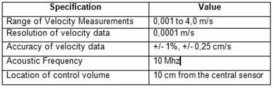
Table 1: Specifications of the FlowTracker 2^® instrumentused to carry out the measuring of this work. 

For the experimental determination with conservative tracer, sodium fluorescein was used due to its availability in the local market, its low environmental impact and its easy handling, without representing any danger to the operators. The tracer minimum mass to be injected was estimated by using Eq. 8, which represents closed-closed boundary conditions, for a flow with a Gaussian concentration distribution and low dispersion values [^{3, 20}].

Although this equation does not represent what happens in a river, it was used to estimate the minimum mass to be injected, since with Eq. 5, as the Ct ₀ , value is not known, it is not possible to calculate this mass. For the other parameters of Eq. 8, the D _L value calculated using the method of Fischer et al [3] was used, while for the C value, the limit of quantification of 1 µg/L was used, corresponding to the determination of the conservative tracer by molecular fluorescence spectrophotometry. As a safety margin, ten times the calculated amount of tracer was injected [33]. Thus, a mass of 15 grams was used for the low-flow test, and 30 grams for the high-flow test.

The mass of tracer was dissolved in a container with 10 litres of water, and the injection was performed instantaneously at the centre point of the SA section (Figure 4).

Figure 4: Advance the injected tracer plume at the SA site. 

After 20 minutes of injection in SA, sampling began in the SB section (Figure 3), in 15 mL glass vials, every 2 to 5 minutes of time interval for 100 minutes, when the flow rate was high and during 110 minutes when the flow rate was low. The sampling frequency was established on the basis of the mean flow velocity and the maximum velocity (obtained by gauging). The samples were cooled and taken to the laboratory for measurement, using a multimodal microplate reader with fluorescence monochromator, model Synergy® H1 from Bioteck, with a detection limit of 0.001 ug/L.The excitation length was 494 nm and the emission length 521 nm. The standards for the calibration curve were carried out at pH 8, since this value was the river pH in both tests carried out. The natural fluorescence of a water sample was also measured before the injection of the tracer, in order to be discounted from the sample measurements.

Results

The values of flow and hydraulic parameters obtained by gauging with the FlowTracker 2 instrument are shown on The same table displays the value of the dispersion coefficient obtained by means of Eq. 2 with a detailed hydrodynamic characterisation.

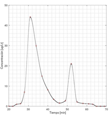
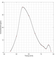
From the concentration data of the samples taken at SB, C-Curves (concentration vs. time) were constructed for each hydrological tested condition (Figures 5 and 6).

Figure5:  CurveC belonging to the test under high flow hydrological conditions. 

Figure 6: Curve C belonging to the test under low flow hydrological conditions. 

The integrals to calculate tm, σ2 from the C-curves (Eq. 3 and Eq. 4, respectively) were obtained using the free distribution program GNU Octave, through polynomial interpolation and integration of the function by Simpson's rule [34].

shows the obtained values of t and as well as the Pe and D _L calculated through Eq. 6 and 7, using the values of U from and L equal to 1000 m (length of the stretch under study).

A tracer recovery of 75% (high flow test) and 73% (low flow test) is observed. The failure to recover the entire mass may be due to the tracer being absorbed by materials, sediments, plants or organisms deposited on the riverbed [35]. It may also be due to a fraction of the mass being trapped in the stream, in so-called dead zones, with a negligible rate of exchange with the flow.

Discussion

In general, in the absence of tracer studies or detailed hydrodynamic data, empirical equations based on global hydraulic parameters are used, which have a large scatter between them and do not always fit the real values [^{13, 36, 37, 38, 39}].

For this reason, they should be cautiously used in rivers with certain characteristics different from those to which they had been adjusted. Research agrees that the uncertainty generated by the theoretical estimation of the parameters of the transport equations, such as the longitudinal dispersion coefficient, can lead to erroneous results in the distribution of concentrations and thus drive to the water resource mismanagement like maximum allowable loads or the length of the affected stretch.

and 3 show that under low flow hydrological conditions, the experimental data with tracer, only differed in 13% with respect to the dispersion coefficient calculated by Eq. 2, based on a detailed hydrodynamic characterisation. On the other hand, for the high flow condition, the experimental data were approximately twice as large as those calculated by Eq. 2. The differences obtained are acceptable in comparison with other results available in literature reporting differences of up to 2 orders of magnitude [6, 36, 40, 41, 42].

When comparing the normalised C curves in Eq. 5, with a Pe value calculated with Eq. 2 and with the Pe value given by the tracer test (Figure 7), it can be seen that there is no difference when the t value is not the maximum (the rising and falling edges of the curve are practically the same). On the other hand, the maximum value of Cwhen D is calculated by the tracer method is 33% lower than when calculated with Eq. 2. This means that the concentration of the substance of interest in SB, at a time equal to t _m and with a D _L =12.6 m²/s will be lower than the concentration calculated with a D = 5.93 m²/s.

Depending on the type of study to be carried out in the river, it will be necessary to analyse whether the uncertainty generated with the coefficients obtained by the hydroacoustic technique is acceptable or not.

Figure 7: Comparison of normalised C curves with dispersion coefficient obtained with Fischer el at method [3] (blue line) and tracer method (orange line). 

A more exhaustive tour of the stream revealed that another mixing mechanism in the stream is the pool-riffle mechanism, which could explain the difference in the D _L values between the two methods; however, the difference observed is within the range reported in the literature [^{43, 44}]. Further analysis of this phenomenon may improve the results obtained from the hydrodynamic data. It should be noted that in both tests, Curve C has had a rising edge with a relatively high slope, but a falling edge with a gentler dip. At the same time, each curve showed higher peaks at t=31 min (high flow) and t=55 min (low flow), and lower peaks at t=52 min (high flow) and t=76 min (low flow). As discussed by [5] and [45], this curve coincides with the ADZ (Aggregated Dead Zone) model, i.e. zones where water stays for a longer time, and then enters into the main channel. The shape of Curve C indicates that, during the low flow season, the section has smaller dead zones compared to the high flow behaviour. It is the greater presence of dead zones that makes the dispersion considerably larger with respect to the low flow condition [46].

Conclusions

The Chicamtoltina stream is a resource of special interest in Cordoba province as it flows through one of the most important cities of the region; it receives an important discharge from the WWTP, and it finally flows into another of the province's important rivers due to its tourist activity, the Anisacate river. To protect the ecosystem and the public health of those who use the resource, water quality models are indispensable in order to predict the concentration of substances derived from the discharge this river receives, such as organic matter, pathogenic bacteria and even affected river parameters such as dissolved oxygen.

As mentioned before, the derivation of mixing parameters in water quality models is generally laborious, which leads to estimations with empirical equations that do not often match with the actual values. The literature shows that the longitudinal dispersion coefficient obtained by means of empirical equations presents values with a significant scattering

In this work, the values of the dispersion coefficient were determined in a 1000-metre section, 50 m from the discharge of Alta Gracia WWTP, by using two methodologies that include the usage of both tracers and hydraulic parameters of one section obtained by gauging. Consequently, during the low-flow season, the D _L value was that of 2.32 m²/s according to the Eq. 2 methodology, and 2.01 m²/s due to the use of tracers, i.e. concordant values. However, in the high flow season, the difference was approximately doubled, being D _L equal to 5.93 m²/s for calculation by means of Eq. 2, and 12.8 m²/s for the methodology with tracer. Such a difference is acceptable for this type of test where previous literature reports a variability from 1 to 2 orders of magnitude.Facing this, it is possible to use the integral equation of Fischer et al. [³] in the stream studied, which is based on a detailed hydrodynamic characterisation with hydroacoustic instrumentation, even when it is recommended to analyse whether the uncertainty generated within the concentration due to the DL value obtained with such hydroacoustics is acceptable or not, mainly during the wet season.

Such gauging is routinely implemented and would allow estimating a D _L value at the end of each campaign Although the values obtained from D _L with the hydroacoustic technique are acceptable, even with an observed difference of approximately double in the high flow condition, periodic tests of tracers in the system are recommended, to analyse the differences between the results of the two methodologies. From the analysis carried out, it is concluded that this coefficient can be estimated for other flow conditions where no tracer test is available, but gauging has been carried out using modern techniques.

Acknowledgements

The authors would like to thank the Science and Technology Secretariat of the National University of Cordoba that subsidized the research project Consolidate 2018-2021 "Optimization of the determination of the Chicamtoltina stream (Alta Gracia)", in the framework of which this work was carried out.