II. Cahn-Hilliard equation

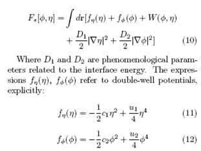
The Cahn-Hilliard equation was developed in 1958 to model the phase separation process of a binary mixture 16. This approach has been extended to many other branches of science as dissimilar as polymer systems 17, population growth 18, image processing 19, and structures formed at the bottom of a river 20, among others. The Cahn Hilliard model is a minimalist approach that contains the elements that are essential to description of the dynamics and the equilibrium properties of a wide variety of systems. The general scheme of the Cahn-Hilliard equation is the following:

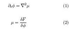
Where represents the chemical potential and F the free energy functional that describes the system under study. Particularly for a binary system, the expression of free energy is given by:

Here, is the order parameter representing the local density of the components. Phase separation occurs during the cooling of the system, from a disorderly, high-temperature state, to an ordered low- temperature state consisting of two phases. The dynamics are controlled by a specic length L, which increases with a power law in time L(t) t(1=3) ²⁰. This Law of Growth implies an extremely slow speed at advanced times during phase separation, with a speed in the domains. There is no analytical solution of the Cahn-Hilliard equation for all time, thus numerical methods are required for resolution. A wide variety of algorithms have been developed to solve the Cahn-Hilliard equation numerically. An extensive analysis of the di erent methods developed can be found in the reference section ²². The traditional method is the cell dynamics method (CDS), whose advantages and disadvantages are discussed in the next section.

III. CDS method

The standard method for numerical resolution of the Cahn-Hilliard equation is the cell dynamics simulation (CDS) method 23. This method corre- sponds to a Euler numerical scheme. The conver- gence of the Euler algorithm strongly depends on the time discretization employed in. Above a certain value of, the system is numerically unstable, presenting "chess-board" instabilities. Consequently, the CDS algorithm is subject to the tmaxx4 23 restriction, where is the spatial discretization. For 1 values, the CDS method provides good convergence, although it requires excessive computational time. On the other hand, in the case of Cahn-Hilliard n = 1=3, coars- ening systems present evolution of their characteristic length L(t) and shape L(t) ' tn. This growth characteristic has a very slow domain growth speed associated with long times. It would be ideal to have a numerical scheme that provided good convergence and allowed varyiation of the time steps, adapting it to the coarsening process. As we saw in the previous equation, the CDS method cannot ful

l this requirement since is limited.

IV. Eyre algorithm

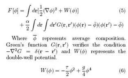
The algorithm developed by Eyre for gradient systems has the advantage of being unconditionally stable for every 15. The algorithm guarantees stability if the free energy functional F is divided into its contractive FC and expansive FE parts. The contractive term is evaluated implicitly and the expansive term, explicitly. The numerical scheme for resolution of the Cahn-Hilliard equation is the following:

Here, the C and E superscripts indicate division of the free energy into contractive and expansive. The stability condition is guaranteed if max is ful lled, where Eand are the eigenvalues of the Hessian matrices of the expansive part of the energy and of the total energy, respec- tively. Implementation of the Eyre algorithm for a specic system requires evaluation of the free en- ergy that characterizes the system.

V. Eyre algorithm applications to block-copolymer systems

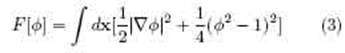
In this section, we will develop the Eyre numerical scheme for the Ginzburg-Landau free energy functional of a diblock copolymer system. In a diblock copolymer system the expression of free energy is the following 25, 26:

The mesoscopic order is the result of competition between a short-range attractive interaction, corresponding to the gradient term of the equation, and a long-range repulsive interaction, corresponding to the long-range term that is imposed to avoid phase macroseparation, and to set the copolymer periodicity. The characteristic wavelength.

After dividing the energy into its contractive and expansive terms, in accordance with the division proposed in the previous section, and evaluating the expansive part explicitly and the contractive part, implicitly, we obtain:

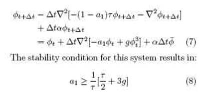
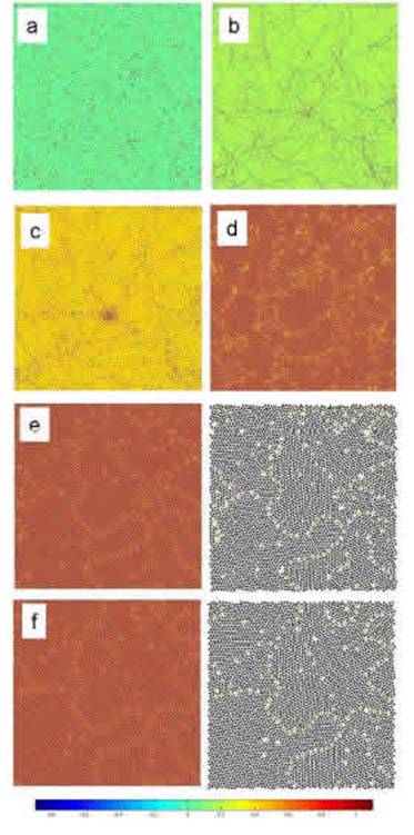
Figure 1: Time evolution of the copolymer system. Simulation data: 1024x1024 grid with spatial discretization x = 0:5 and periodic boundary conditions. For the copolymer, g = 1; = 1; = 0:1 and = 2:1 was used. Time (a) t = 0, random initial condition, (b) t = 50 (c) t = 100, (d) t = 500, (e) t = 1000, (f) t = 5000. Note that the location and identication of topological defects of the hexagonal patterns have been included in the last two images. 

Figure 2: Size of the domains L vs. time t. The results show a growth law Lt0:330:01 in good agreement with the previous results. The plotted values correspond to an average over 10 simulations. 

VI. CDS vs. Eyre comparison

The CDS algorithm registers good convergence in the numerical resolution of the Cahn-Hilliard equation. However, its e ectiveness is limited by requiring an extremely small time step t. In this section, the CDS and Eyre algorithms for numerical resolution of the Cahn-Hilliard equation for modeled diblock copolymer systems are compared with the Ginzburg-Landau free energy functional system, according to the result obtained in the previous section. The time evolution of a 2D system with a 1024x1024 grid with spatial discretization of x = 0:5 periodic boundary conditions was simulated. A pseudo-spectral method was used for spatial derivatives 27. For the copolymer, g = 1; = 1; = 0:1 and = 2:1 were used. The bulk equilibrium structure corresponds to a BCC formation of spheres, while in 2D systems it corresponds to an hexagonal arrangement, as can be seen in Fig. 1, where the time evolution of the system is illustrated, starting from a disordered state. The value t = 0:03 was assigned to the CDS method.

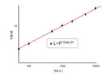
The evolution of the system and the growth of the size of the domains was measured using standard image processing techniques to identify the center of each disk in the hexagonal pattern. A Delaunay triangulation 28 was then used to determine the inter-bond orientation between near-neighbor disks m(r). Finally, the average domain size L(t) was obtained through the orientational correlation length1. The results are presented in Fig. 2 obtaining a growth law L mt0:330:01 in good agreement with the previous results. In order to compare these methods, the diference between the numerical solutions obtained by each algorithm for the above-mentioned system was calculated. The solution of the CDS method was taken as a reference. The energy of the system was calculated at each time step. Remember that in gradient systems the energy decreases as time progresses. The solutions were compared to equal values of free energy, and the E error associated with the Eyre method was calculated by expressing 30:

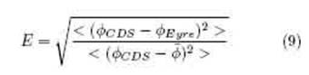
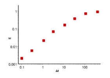
by the Eyre method. The notation indicates an average over all points of the spatial grid. The results for df erent t values of the Eyre algorithm are presented in Fig. 3, where the error value for a given t corresponds to an average over 100 comparisons of the Eyre solution with regard to the solution taken as a reference to equal energy values.

For a three percent bounded error, the Eyre algorithm was 120 times faster than the CDS method.

Figure 3: Calculation of the error E associated with the simulations performed for di erent t time discretizations, compared with the CDS system used as a reference according to equation 9. The plotted values correspond to an average over 100 simulations.  

VII. Free energy of a copolymersolvent system

We can express the free energy of a copolymersolvent ternary system based on the order parameters and -, where - represents the composition of the copolymer mixture, and, the solvent 31, 32. The energy is composed of a shortrange term Fs and a long-range term the short-range term is the following:

The expression above is related to the parameter that represents the copolymer. The bi parameters of the interaction potential characterize the interactions between block copolymers and the solvent. The evolution of the order parameters - and represents the evolution of the copolymer and the solvent, respectively. Time evolution results in a set of coupled di erential equations for conserved order parameters.

VIII. Eyre algorithm for the Cahn Hilliard equation

The Eyre algorithm previously developed for a copolymer system can be adapted to solve the Cahn-Hilliard equation set that models the time evolution of the copolymer and solvent equations 15 and 16. The expression of the algorithm is the following:

IX. Numerical simulations

In order to evaluate the numerical resolution obtained by the Eyre method, the time evolution of a 2D copolymer-solvent system was simulated. The system was simulated with a 512x512 grid with x = 0:5;t = 1:5 and periodic boundary conditions for both order parameters. A pseudo-spectral method was used for spatial derivatives 27.

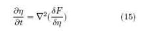
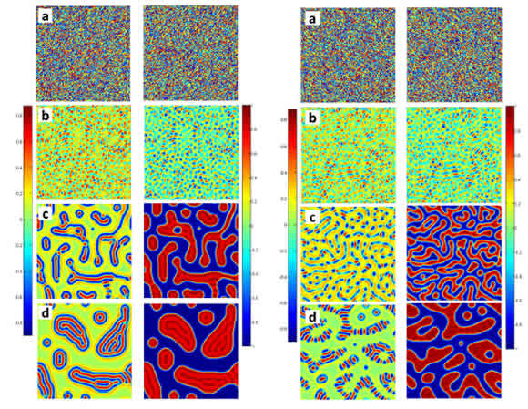
Figure 4-5: Time evolution of the copolymer-solvent system. The gures show the order parameter of copolymer - on the left and the order parameter of solvent on the right. Simulation data: system with a 512x512 grid with x = 0:5;t = 1:5 and periodic boundary conditions for both order parameters. c2 = 0:1; u2 = 1;D2 = 1; = 1; = 0 was used for the copolymer. For this set of parameters the structure corresponds to a lamellae structure. c1 = 0:3; u1 = 1;D1 = 0:5 was used for the solvent. The interaction parameters were b1 = 0:07; b2 = 0:3; b3 = 0; b4 = 0:1. Times: (a)t = 0, (b)t = 10, (c)t = 1000, (d)t = 10000. Figure 5: Time evolution of the copolymer-solvent system. The gures show the order parameter of copolymer - on the left and the order parameter of solvent on the right. Simulation data: system with a 512x512 grid with x = 0:5;t = 1:5 and periodic edge conditions for both order parameters. c2 = 0:1; u2 = 1;D2 = 1; = 1; - = 0 was used for the copolymer. For this set of parameters the structure corresponds to a lamellae structure. c1 = 0:3; u1 = 1;D1 = 0:5 was used for the solvent. The interaction parameters were b1 = 0:03; b2 = 0:3; b3 = 0; b4 = 0:1. Times: (a)t = 0, (b)t = 10, (c)t = 1000, (d)t = 10000. 

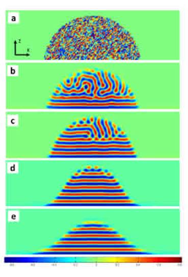
Figure 6: Time evolution of copolymer nano-drops on a rigid substrate. The composition of the copolymer is shown in the x, z plane. Simulation data: system with a 512x512x256 grid with x = 0:3;t = 1:5 and periodic boundary conditions in the x and y directions and no ow in the z direction. c2 = 0:1; u2 = 1;D2 = 1; = 1; - = 0 was used for the copolymer. For this set of parameters the structure corresponds to a lamellae structure. c1 = 0:3; u1 = 1;D1 = 0:5 was used for the solvent. The interaction parameters were b1 = 0:03; b2 = 0:3; b3 = 0; b4 = 0:1. Times: (a)t = 0, (b)t = 1000, (c)t = 10000, (d)t = 100000. 

Figure 7: (a) Nano-droplet structures obtained for a bulk phase copolymer of lamellae. (b)AFM image. Nano-droplet of copolymer in lamellae phase obtained by the dewetting process. The image shows the stepwise shape of the droplet induced by competition between the surface tension on the liquid surface and the lamellae structure, forming the copolymer droplet. The image was extracted from the work of Croll et al. 33. 

this set of parameters, the structure corresponds to a lamellae structure. For the solvent, c1 = 0:3; u1 = 1;D1 = 0:5 was used. The interaction parameters were b1 = 0:07; b2 = 0:3; b3 = 0; b4 = 0:1. Fig. 4 illustrates the time evolution of the copolymersolvent system phase separation. The b1 parameter determines the preference or anity of the solvent for one of the copolymer blocks. For the value b1 = 0:07, there is a strong anity with one of the blocks, which results in the formation of copolymer micelles. It should be noted that in most parts of macrodomains, the lamellar domains tend to be parallel to the macrophase interfaces and the domains are surrounded by a thin layer of one block. The decrease in the b1 value to a b1 = 0:03 value is illustrated in Fig. 5. A lower b1 value results in similar anity between the copolymer blocks and the solvent. As seen in Fig. 5, the interface of the copolymer domains is uniformly composed by both blocks. For this value the stripe domains emerge perpendicularly to the macrophase interfaces. Thus a clear morphological transition is brought about by changing the interaction parameter b1. Parameter b1 allows the interaction between the solvent and the copolymer blocks to be modeled. The morphological change occurs at about b1 = 0:04. This behavior coincides qualitatively with the experimental results 32. To illustrate this point we simulate the formation of a nano-drop on a rigid substrate. To simulate the temporal evo- lution of a copolymer droplet deposited on a rigid substrate, the air copolymer system was modeled as a ternary system (solvent copolymer), where the air was treated as a bad solvent. The system was simulated with a 512x512x256 (x; y; z) grid with x =y =z = 0:3 and t = 1:5. Periodic boundary conditions in the x and y directions and no ux in the z direction were used. The Eyre algorithm developed in the previous section was used for time evolution, and spatial derivatives were resolved using a pseudo-spectral method. Starting from a disordered state, the time evolution is illustrated in Fig. 6. The nal equilibrium structure is illustrated in Fig. 7. Experimental work in the literature shows a similar formation of structures within the nano-droplets. Fig. 7, insert b, shows the image of a nano-droplet obtained by the dewetting process of a diblock polystyrene-polymethyl methacrylate (PS-PMMA) copolymer in the lamellae phase. Details can be found in the work of Croll et al.33. The images show good qualitative agreement with the nano-drop obtained by numerical simulation.