


 Inglés (pdf)
 Articulo en XML
 Referencias del artículo
 Enviar articulo por email
 Citado por SciELO
  Similares en
SciELO
Similares en
SciELO 
 Permalink
I. Introduction
Research on the dynamics of pulsatile ows through constricted regions has multiple applications in biomedical engineering and medicine. Cardiovascular diseases are the primary cause of death worldwide (accounting for 31% of total deaths in 2012) [1]. More than half of these deaths could have been avoided by prevention and early diagnosis. Atherosclerosis is characterized by the accumulation of fat, cholesterol and other substances in the intima layer, creating plaques which obstruct the arterial lumen. Atherosclerotic plaque ssuring and/or breaking are the major causes of cardiovascular stroke and myocardial infarct. Several factors leading to plaque complications have been reported: sudden increase in luminal pressure [2], turbulent uctuations [3], hemodynamic shear stress [4], vasa vasorum rupture [5], material fatigue [6] and stress concentration within a plaque [7]. As most of these factors are ow dependent, understanding how a pulsatile ow behaves through a narrowed region can provide important insights for the development of reliable diagnostic tools.
Flow alterations due to arterial obstruction (i.e. stenosis) and aneurysms have been reported in the literature [8-11]. Simplied models of stenosed arteries have used constricted rigid tubes [12-15]. At moderate Reynolds numbers, the altered ow splits at the downstream edge of the constriction into a high-velocity jet along the centreline and a vortex shedding zone separating from the inner surface of the tube wall (recirculation ow). Increasing Reynolds numbers lead to a transition pattern and ultimately, turbulence. Several experimental studies have been reported. Stettler and Hussain [16] studied the transition to turbulence of a pulsatile ow in a rigid tube using one-point anemometry. However, one-point anemometry fails to account for diferent ow structures which may play an important role at the onset of turbulence. Peacock [17] studied the transition to turbulence in a rigid tube using two-dimensional particle image velocimetry (PIV). Chua et al [18] implemented a three-dimensional PIV technique to obtain the volumetric velocity eld of a steady ow.
The work of Ahmed and Giddens [19,20] studied the transition to turbulence in a constricted rigid tube with varying degrees of constriction using twocomponent laser Doppler anemometry. For constriction degrees up to 50% of the lumen, the au- thors found no disturbances at Reynolds numbers below 1000. This study was not focused on describ- ing vortex dynamics; however, the authors reported that turbulence, when observed, was preceded by vortex shedding.
Several authors carried out numerical studies. Long et al. [15] compared the ow patterns produced by an axisymmetric and a non-axisymmetric geometry, nding that ow instabilities through an axisymmetric geometry was more sensitive to changes in the degree of constriction. The work of Isler et al. [21] in a constricted channel found the instabilities that break the symmetry of the ow. Mittal et al. [22] and Sherwin and Blackburn [23] studied the transition to turbulence over a wide range of Reynolds numbers. Mittal et al. used a planar channel with a one-sided semicircular constriction. They found that downstream of the constriction the ow was composed of two shear layers, one originating at the downstream edge of the constriction and the other separating from the opposite wall. For Reynolds numbers above 1000, the authors reported transition to turbulence due to vortex shedding. Moreover, they found through spectral analysis that the characteristic shear layer frequency is associated with the frequency of vortex formation. Sherwin and Blackburn [23] studied the transition to turbulence using a three-dimensional axisymmetric geometry with a sinusoidal constriction. Based on the results of linear stability analysis, the authors reported the occurrence of KelvinHelmholtz instability. This rea rms that instabilities involving vortex shedding take place in the transition to turbulence.
Finally, several studies compared experimental and numerical results. Ling et al. [24] compared numerical results with those obtained by hot-wire measurements. As mentioned above, onedimensional hot-wire measurements cannot be used to identify ow structures. Grith et al. [25], using a rigid tube with a slightly narrowed section resebling stenosis, compared numerical results with experimental data. Using stability analysis by means of Floquet exponents, they demonstrated that the experimental ow was less stable than that of the simulated model. For low Reynolds numbers (50 the authors found that a ring of vortices formed immediately downstream of the stenosis and that its propagation velocity changed with the degree of stenosis. The work of Usmani and Muralidhar [26] compareed ow patterns in rigid and compliant asymmetric constricted tubes for a Reynolds range between 300 and 800 and Womersley between 6 and 8. The authors reported that the downstream ow was characterized by a high velocity jet and a vortex whose evolution was described qualitatively. The aforementioned studies highlight the signicance of studying vortex dynamics, since vortex development precedes turbulence, and ultimately, contributes to the risk of a cardiovascular stroke.
The aim of this work is to characterize vortex dynamics under pulsatile ow in an axisymmetric constricted rigid tube. The study was carried out both experimentally and numerically for di erent constriction degrees and with mean Reynolds num- bers varying from 385 to 2044 andWomersley num- bers from 17 to 50. The results show that the ow pattern in these systems consists primarily of a cen- tral jet and a vortex shedding layer adjacent to the wall (recirculation ow), consistent with the literature. By tracking the vortex trajectory it was possible to determine the displacement of vortices over their lifetime. Vortex kinematics was described as a function of the system parameters in the form of a dimensionless scaling law for maximum vortex displacement.

II. Materials and methods
i. Experimental setup
The experimental setup (Fig. 1 (a)) consisted of a circulating loop and a Digital Particle Image Velocimetry (DPIV) module capable of obtaining videos and processing velocity melds. The circulating loop consisted of a programmable pulsatile pump (PP), a reservoir (R), a ow development section (FDS) and a tube containing an annular constriction (CT). The tube with the annular constriction (CT) consisted of a transparent acrylic rigid tube of length L = 51:0 0:1 cm and inner diameter D = 2:6 0:1 cm. The annular constriction consisted of a hollow cylinder 5 1 mm in axial length, which was mtted inside the rigid tube. Keeping the outer diameter of the annular constriction mxed at 2.6 cm, i.e., equal to the inner diameter of the rigid tube, its inner di- ameter was changed to achieve di erent degrees of constriction. Tests were carried out using annular constrictions with inner diameters d0 = 1:6 0:1 cm and d0 = 1:0 0:1 cm, equivalent to degrees of constriction relative to D of 39% and 61%, respectively. A cross-sectional scheme of the constriction geometry is shown in Fig. 1 (b), along with the coordinate system used throughout the study. The radial direction is represented by r and the axial direction by z, with r = 0 coinciding with the tube axis and z=0 with the downstream edge of the constriction. Within this axis representation, the downstream region is dened by z >0 values and the upstream region is dened by z < 0 values. Finally, this constricted tube (CT) was placed inside a chamber lled with water, so that the refraction index of the uid inside the tube matched that of the outside uid.
The tube inlet was connected to the pulsatile pump via a ow development section (FDS), and its outlet was connected to the reservoir. The ow development section was designed to ensure a fully developed ow at the tube inlet and consisted of two sections: rst, a conical tube of 35 cm in length whose inner diameter increased from 1 cm to 2.6 cm to provide a smooth transition from the outlet of the pump. Secondly, an acrylic rigid tube of inner diameter D and length of 48D connected to the constricted tube (CT). The reservoir (R) was used to set the minimum pressure inside the tube, which was set as equal to atmospheric pressure in the experiments.
The system was lled with degassed water and seeded with neutrally buoyant polyamide particles (0.13 g/l concentration, 50 m diameter, DANTEC). The DPIV technique was used to obtain the velocity eld [27,28]. A 1WNd:YAG laser was used to illuminate a 2 mm-thick section of the tube. Images were obtained at a frame rate of 180 Hz over a period equivalent to 16 cycles, using a CMOS camera (Pixelink, PL-B776F). The velocity meld wasnally computed using OpenPIV open-source software with 32 32 pixel2 windows and an overlap of 8 pixels in both directions.
The region of interest was de ned as -0.5< r=D <0.5, 0< z=D <1.5. Within this region no turbulence was observed, as conrmed by spectral analysis of the velocity elds. This observation is also consistent with previous observations [17,24,29]. Due to the pulsatility and the absence of turbulence, it was possible to consider each cycle as an independent experiment, using the ensemble average over all 16 cycles to obtain the nal velocity elds.
For each degree of constriction di erent experiments were carried out, varying the ow velocity at the tube inlet. The pulsation period and the shape of the velocity as a function of t, in z = 0 and r = 0, shown in Fig.1 (c), remained unchanged throughout the experiments. Pulsation period and peak velocity can be related to the Womersley and Reynolds numbers, respectively. The Womersley number, is dened as = D 2 q2 f , where fis the pulsatile frequency and the kinematic viscosity of water ( = 1:0 10 summarized in table 1.


Figure 2: Normalized displacement of piston yp for Reu=505 (diamond green), Reu=820 (blue circles), Reu=1187 (red squares), Reu=1625 (black plus sign).
The pulsatile pump (PP in Fig. 1 (a)) generated dierent ow conditions at the tube inlet, [30]. The pumping module consisted of a step-by-step motor driving a piston inside a cylindrical chamber. The control module contained the power supply for the entire system and an electronic board, programmable from a remote PC by means of custom software. The piston motion was programmed using the pump settings for pulsatile period, ejected volume, pressure and cycle shape. The piston motion of the programmable pump is shown in Fig. 2 in normalized units of displacement and time. Figure 2 shows that the piston motion, and hence the pulsatile waveform, are comparable among all Reu values, meaning that the inlet conditions are equivalent for all the experiments.

Figure 3: Upstream velocity proles for (a) Reu=820, (b) Reu=1187 and (c) Reu=1625. Proles are located at z1=-1.25D (blue circles), z2=-0.75D (red triangles) and z3=-0.25D (black plus sign).
Finally, the condition of fully-developed ow at the upstream region was veried. The entrance length is usually estimated as L m0:05ReD. According to the work of Ku [31], the entrance length of a pulsatile ow with 10 corresponds to the upstream mean Reynolds over a whole cycle, mReu, giving L m0:05 mReuD. In our setup, the ow development section measures 48D, Reu <1000 and >10 for all experiments, which makes it reasonable to assume a fully-developed ow. Nevertheless, velocity proles were studied for Reu values of 820, 1187 and 1625 in order to ensure developed ow condition. Proles are taken from a 1:5D length window upstream of the constriction, atxed locations z1 = ii. Numerical simulation Three-dimensional numerical simulation using COMSOL software enabled comparison between the experimental data and the study of param- eter congurations not achieved experimentally. This entailed solving time-dependent Navier-Stokes equations under the incompressibility condition. The inlet condition was dened as normal in ow and taken from Reu=820 and Reu=1187 experimental data in the upstream region, where the ow is developed. In order to do this, a fourth-order Fourier decomposition of the experimental ow rate was carried out. The Fourier expansion yields vz(t) = a0 2 +P4 n=1 (ancos (2nft) + bnsin (2nft)) with coecients (10 time increasing steadily from 0 to 1 in 0.6 seconds. Figure 4(a) shows the axial velocity at the centreline at the downstream edge of the constriction, and presents good agreement with its experimental analogue shown in Fig. 1 (c). Outlet conditions were set to p = 0, p being the diference between the outlet pressure and atmospheric pressure, disabling the normal ow and back ow suppression settings.
No-slip conditions were imposed on the inner sur- face of the tube wall or the constriction. A scheme of the geometry of the constricted tube used in the numerical analysis is shown in Fig. 4(b). The simulations were initialized with the uid at rest and were run for 20 periods. The rst 4 periods were discarded in order to exclude transient efects. The step size for the data output was selected to be the same as for the experiments.
The mesh elements were tetrahedrons except those close to the no-slip boundaries, which were prismatic elements. This was done automatically by COMSOL, based on the boundary requirements. A COMSOL predened physics-controlled mesh was built, enabling settings that allowed the element size to adapt to the physics at specic regions. A cross-sectional view of the tube and the mesh elements is shown in Fig. 4 (c). Figure 6 compares numerical and experimental velocity proles in order to validate numerical results. Pro es are located upstream.
III. Results and discussion
i. Flow pattern
The velocity at the centreline, r = 0, at the downstream edge of the constriction, z = 0, as a function of time (see Fig. 1(c)) was used to establish the time reference for all the experiments. The decelerating phase (diastolic phase) was dened as 0 < t < 0:5T and the accelerating phase (systolic phase) as 0:5T < t < T. Figures 7 and 8 show the temporal ow patterns obtained from the experimental data corresponding to Re=654, 1002, 1106, 1767 and 2044, while Fig. 9 shows the patterns obtained via simulation. Figures 7(a), 8(a) and 9(a) show the ow evolution at times 0.25 T, 0.5 T, 0.6 T and 0.9 T. Some features were common to all the experiments and numerical results. During the accelerating phase two main ow structures can be distinguished: a central, high-velocity central jet and a recirculation zone between the former and the inner surface of the tube wall, with vortices developing in the latter. In Figs. 7, 8 and 9, the central jet is shown in blue and the recirculation zone in red. The central jet is distinguished from the recirculation zone by having vorticity values below the threshold of 30% of the maximum of the absolute value of vorticity in each timestep. The aim of this criterion is to separate regions approximately rather than give their precise location. Within the recirculation zone, vortices separated from the wall and travelled along the tube.
Other features are dependent on the Reynolds number. For instance, for Re = 654 (Fig. 7 (b)) the vortex had already developed at the rst half of the decelerating phase and propagated until the beginning of the accelerating phase, as suggested by the dashed lines. At this stage, the thickness of the recirculation zone is approximately equal to h. During the accelerating phase, the thickness of the recirculation zone began to decrease as that of the central jet increased. Toward the end of this phase, the central jet was thicker and the previous vortex had almost entirely dissipated, while a new vortex had begun to develop in the vicinity of the constriction (z=D < 0:2). For Re = 1106(Fig. 7 (c)), the ow presented the same characteristics as for Re = 654. Here, the vortex travelled faster during the entire cycle and the recirculation zone was 27% thicker. This is ascribed to the increment in the peak velocity of the central jet and the consequent increase in shear stress, leading to enlargement of the recirculation zone and an increase in radial velocity.
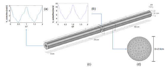
Figure 4: (a) Axial inlet velocity at r = 0; corresponds to Reu = 1187; (b) axial velocity at r = 0 and z = 0; corresponds to Re = 1106; (c) schematic drawing of the ow development section and the axisymmetric constricted tube; (d) cross sectional view of the mesh.
At Re = 654 and Re = 1106 two vortices were observed in the region of interest over one pulsatile period (Figs. 7(b) and (c)). In the case of Re = 1106 (Fig. 8 (b)), only one vortex was observed over one period. This di erence arose because the vortex propagates at lower velocities for lower Reynolds values, then it is expected that two vortices will be observed in the region of interest, which were shed in consecutive pulsatile periods. For Re = 1106 at the beginning of the accelerating phase, the central jet decreased in thickness and the recirculation zone became enlarged to occupy almost the entire tube section at z=D 1. This can be attributed to a marked deceleration of the central jet at the start of the accelerating phase. Due to mass conservation, the radial velocity is expected to increase, leading to enlargement of the recirculation zone. This is also consistent with that reported previously by Sherwin [23].
At Re = 1767 (Fig. 8 (c)), the vortex developed and propagated faster than in the previous cases, and a secondary vortex was observed. In the decelerating phase, the vortex reached its maximum size and almost escaped from the region of interest. When the velocity of the central jet at the constriction was near its minimum, the vortex left the region of interest and the rest of the ow became disordered. In the accelerating phase, the vortex developed earlier than at lower Reynolds numbers. Comparison of Figs. 7 and 8 illustrates how the
ow pattern changed with the degree of constriction. While in Fig. 7 the vortex travelled without a substantial change in size, Fig. 8 (b) shows a sharp change in vortex size, measured radially, and Fig. 8 (c) shows that the vortex had almost en- tirely dissipated at t = 0:5T. Moreover, due to the reduction in d0 (Fig. 8) the velocity of the central jet was higher, and the recirculation zone became enlarged with increasing z, which explains the increase in vortex size. This is consistent with that reported by Sherwin et al. [23] and Usmani [26]. Enlargement of the recirculation zone was present throughout the experiments. This could be explained in terms of circulation, as pointed out in the work of Gharib et al. [32] which studies the ow led by a moving piston into an unbounded domain. This work determined that a vortex forms up to a limited amount of circulation before shedding from the layer where it was created. The main difference from our work consists in the connement that the walls impose on the vortex. The result is that a vortex which sheds with a certain amount of circulation enlarges in the axial direction. This mechanism can also explain the generation of a secondary vortex. Specically, the vortex sheds after a precise amount of circulation is reached. Then any excess of circulation generated goes to a trail of vorticity behind the vortex, eventually identied as a secondary vortex.

Figure 5: Behavior comparison for three meshes: 180958 elements (Mesh 1), 351569 elements (Mesh 2) and 951899 elements (Mesh 3). (a) Axial velocity at r = 0, z = 0 vs time and (b) Velocity proles in downstream location z = 0:5D at 0.25T, 0.5T, 0.75T and T.
Finally, experimental and numerical results were compared in order to validate the simulation. Figure 9 shows the evolution of the simulated ow at Re = 654 and Re = 1106. Comparison of Fig. 9 with Fig. 7 conrms similar behaviour for the experimental and simulated ows. The main structures, i.e. the central high-velocity jet and recirculation zone, were satisfactorily reproduced by numerical simulation.
ii. Vortex propagation
Vortex propagation was studied by measuring vortex displacement as a function of time along one pulsatile period. To this end, the study region was constrained to 0:3 < r=D < 0:5 in order to isolate the vortex fraction forming in the superior wall of the tube. In this region vorticity values of the vortex are positive. For each time frame, the vorticity eld was used to extract the vortex position. Then, in each frame, all vorticity values below a threshold of 30% of the maximum vorticity value were disregarded in order to obtain the ltered vorticity meld (r; z). The vortex position was then calculated as (r; z) = P(r; z) (r; z). The vortex propagation was along z and is specied ings. 7, 8 and 9 by a black dashed line. This aforementioned method enables us to track the vortex andnally to measure the vortex maximum displacement, which will be discussed in the next subsections.
iii. Numerical results for varying Womers- ley number
Maximum vortex displacement was dened as z=D. Position zis where vorticity becomes lower than 30% of the maximum vorticity and is measured from z0, the position where the vortex formed. Position z0 was dened as the location of the vortex centre before it sheds. The dependence of the vortex displacement over its lifetime on , or f, was studied numerically for xed values of Re = 654 and Re = 1106, and pulsatile frequency values of 0.5 f, 0.75 f, f, 1.5 f and 2 f, where f is the pulsatile frequency tested experimentally. Figure 10 clearly illustrates the dependence of the maximum vortex displacement on . For axed value of Re , as increased, i.e., f increased, the ow behaviour tended to replicate within a smaller region of the tube over a shorter time span. With increasing , vortices tended to have a shorter lifespan and their maximum displacement was therefore smaller. In other words, z=D decreased with increasing pulsatile frequency.
iv. Scaling law
A full description of vortex displacement has been given in previous sections. Specically, the maximum displacement of the vortex was studied; that is, the distance it travels before it vanishes. From our results we propose a scaling law which summarizes the behavior of z=D as a function of the parameters involved,e and.

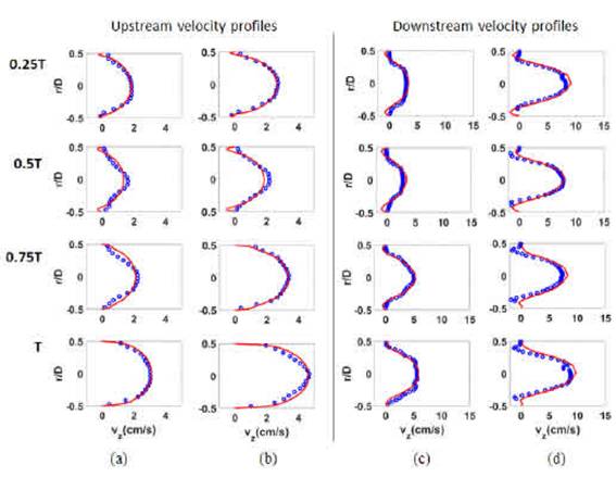
Figure 6: Experimental (blue circles) and numerical (red solid line) velocity proles at upstream location z = for (a) Reu=820, (b) Reu=1187 and at downstream location z = 0:75D for (c) Reu=820, (d) Reu=1187
The physical dimensions for the relevant variables are , D, f and v. Based on the Vaschy Buckingham theorem, it is possible to describe z=D as a function of two independent dimensionless numbers, Re and m, which involve the relevant variables mentioned. Maximum displacement z=D was found to be proportional to ow velocity v (i.e. Re ), and inversely proportional to pulsation frequency f (i.e. 2), suggesting that the data of Fig. 10.
The work of Gharib et al. [32] shows that the developing vortex reaches a threshold of circulation before it sheds. If an excess of circulation is generated, this could lead to the formation of other structures such as secondary vortices. This means that pulsatile frequency f coincides with the shedding frequency of the primary vortex, the one that was tracked. Hence, the parameter Re= 2 can be related to the Strouhal number through Re=2 = 2 d0 D 1 Sr . A discussion of the results in terms of the Strouhal number claries the rela- tion between the oscillatory component of the ow and the stationary component of the ow. For lower values of Re=2, that is, Sr close to 1, stationary and oscillatory components are comparable, which explains a vortex with low to null displacement. The extreme case occurs when the ow oscillates but no vortices are shed. For instance, this could be attained for Reynolds numbers below those used in this work. As Re=2 increases, that is for Sr vortices are shed and travel further before vanishing as a consequence of the stationary component of the ow being greater than the os- cillatory component. Parameter Re=2 also states the kinematic nature of vortex displacement, and by rewritin Re 2 = 2d0v D2f we conclude that z=D depends on kinematic variables and not on viscosity.
Finally, this shows that Eq. 1 can be considered as a scaling law that describes the vortex displacement over its lifetime for any combination of the relevant parameters Re and within the range studied and the constriction shape used. Specically for the dependence on constriction shape, preliminary results with a Guassian-shaped constriction were obtained numerically, giving a di erence below 20% for the maximun vortex displacement for Reu=1187. Vortex dynamics depend on inlet condition shape [23,33]. However, studies are not conclusive regarding the dependence of the vortex maximum displacement on the shape of the inlet condition. Further research is being carried out on this point.

Figure 7: (a) Axial velocity prole at z = 0 and r = 0 and time at which the velocity eld was obtained (red circles); (b) streamlines derived from experimental data for Re = 654, with d0 = 1.6 cm; (c) streamlines derived from experimental data for Re = 1106, with d0 = 1.6 cm. In both cases, red streamlines represent the recirculation zone and blue streamlines the central jet (colours available online only).

Figure 8: (a) Axial velocity prole at z = 0 and r = 0 and time at which the velocit eld was obtained (red circles); (b) streamlines derived from experimental data for Re = 1002, with d0 = 1.0 cm; (c) streamlines derived from experimental data for Re = 1767, with d0 = 1.0 cm. In both cases, red streamlines represent the recirculation zone and blue streamlines the central jet (colours available online only).

Figure 9: (a) Axial velocity prole at z = 0 and r = 0 and time at which the velocity eld was obtained (red circles); (b) streamlines derived from simulation results for Re = 654; (c) streamlines derived from simulation results for Re = 1106. In both cases, red streamlines represent the central jet layer and blue streamlines represent the central jet (colours available online only).
IV. Conclusions
In this work, a pulsatile ow in an axisymmetric constricted geometry was studied experimentally and results were compared with those obtained numerically for the same values of Re and. Af- ter validation of the numerical results, simulations were run over a range of values that could not be tested experimentally, in order to identify trends in flow behaviour with varying.
The ow structure was found to consist of a central jet around the centreline and a recirculation zone adjacent to the wall, with vortices shedding in the latter. The analysis addressed how the vortex trajectory and size changed with the system parameters. Specically, for a xed value of m, vortex size grew with decreasing d, and vortex displacement was larger for increasing Re values. The dependence on was such that as increased, the behavior of the ow was reproduced in a shorter extension of the tube. The vortex trajectory was tracked and its displacement over its lifetime determined. Results showed that vortex displacement over its lifetime decreased with increasing . The analysis led to a scaling law establishing linear dependence of the vortex displacement on a dimensionless parameter combining Re and , namely Re=2 . Moreover, this parameter was found to be proportional to the inverse of the Strouhal number. This directly relates the vortex behavior to the ratio between the pulsatile component and the stationary component of the flow.

Figure 10: Dependence of the dimensionless maximum vortex displacement on. Experimental results in blue squares and numerical results in red circles (Re = 654) and red triangles (Re = 1106).
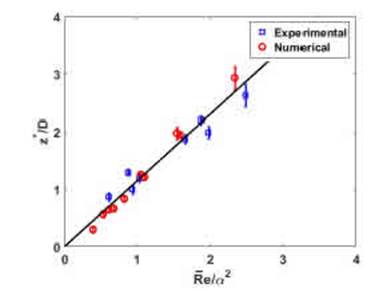
Figure 11: Dimensionless maximum vortex displacement, z=D, as a function of the dimensionless parameter Re=2 for experimental data (blue squares) and numerical data (red circles).
As seen from the medical perspective on the issue of stenosed arteries, these results provide insight into vortex shedding and displacement in a simplied model of stenosed arteries. This becomes crucial since vortex shedding precedes turbulence, and turbulence is related to plaque complications which may nally lead to cardiovascular stroke. The authors encourage further research into the behaviour of vortices over a wider range of parameters, including diferent constriction shapes and sizes.
Acknowledgements
This research was supported by CSIC I+D Uruguay, through the I+D project 2016 \Estudio dinamico de un ujo pulsatil y sus implicaciones hemodinamicas vasculares", ANII (Doctoral scholarship POSNAC-2015-1-109843), ECOSSUD (project reference number U14S04) and PEDECIBA, Uruguay. The manuscript was edited by Eduardo Speranza.

