i. Spatially resolved 3D imaging

The fundamental challenges in acquiring spatiallyresolved 3D images from the bulk, i.e. the inner part, of a dense granular system using electromagnetic waves include:

(a) The amount of information that has to be gathered from the sample to create a full threedimensional image. If our desired resolution is m micrometer per pixel and our region of interest has a side length of l micrometer, we need to take images with (l/m)² pixels. Now, if we want to measure a cubic volume of (l/m)³ voxels (the 3D equivalent of pixels), we need αl/m images. The prefactor α ranges from 1 for RIMS, where we can√ directly acquire neighboring slices, to 2 as fre-quently used in X-ray tomography. In practice, l/m typically ranges from 500 to 2000. Acquiring this number of individual images is time-consuming. Therefore, 3D imaging techniques are well suited to study static granular packings but will have problems imaging fast granular dynamics where particles move with speeds above ≈ 0.01 diameters per second. This definition encompasses granular phenomena such as dynamical heterogeneities in slowly driven systems, shear in split bottom cells, dense flows in chutes, silos or down inclined planes, avalanches and segregation in rotating drums, or granular gases driven by electromagnetic shakers.

This imaging speed problem does not occur if the dynamic process can be repeatedly stopped and restarted, such as with grain breakage under load (64, 65), or if the dynamics happens on the timescales of several hours, i.e. much longer than the typical acquisition times described below. Examples for this situation include creep under constant load (66), root growth (67,68) or the formation of ice lenses in frozen soil (67).

(b) The interaction between the waves and the material the grains are made from should be material-specific and enable the localization of the measured signal. The latter condition is met by some types of absorption or local excitation. In contrast, refraction will not work for imaging because it will occur at all grain interfaces the waves encounter. In consequence, the grains at the container boundary will blur any image of deeper layers.

In order to make the subsequent discussion more substantial, we will now focus on X-ray tomography (69) as imaging modality. Regarding (A): First, each imaging technique must strike a balance between the signal-to-noise ratio (SNR) of the images and the time allowed to acquire an individual image. We can measure the SNR by taking a series of static images and computing the gray value distribution of a pixel in the region of interest. The mean of that distribution is the signal we are interested in, and the standard deviation around that mean is the measure for the noise in any individual image. Because the generation of photons, their interaction with the sample material, and their probability of being detected in the camera are all stochastic processes, the number of photons detected by any given camera pixel will follow a Poisson distribution. For Poisson distributions the SNR is proportional to N, where N is the number of photons.

Due to its relevance for our own vision, mankind has developed quite powerful sources of photons in the optical range. This allows optical high speed cameras to acquire hundreds of thousands of images per second at good quality. Photon sources for Xrays have only been explored since the work of Wilhelm R¨ontgen in 1895. As discussed below, most of the available sources are comparatively dim. Combined with the fact that the imaging mechanism is absorption, which further decreases N, a reason able SNR often requires exposure times which make it impossible to image moving objects without motion blur. Even worse, the high dynamic range necessary for absorption imaging will often require the acquisition of n images of the non-moving sample. Averaging those images will then increase the SNR by n, however at the cost of increasing the acquisition time by a factor of n.

Figure 3 Challenges in X-ray imaging. a) Material mixtures, which do not differ significantly in their attenuation coefficients, can only be segmented by error-prone subsequent image processing. The panel shows as an example a cross-section through a container with plant roots in soil using two different algorithms to identify the root: green areas are roots found by both algorithm, red and yellow areas are found by only one of the two (adapted from (62)). b) Beam hardening arising from the energy dependent attenuation of X-rays: The photon spectrum in front and behind a sample differ qualitatively. This change is not accounted for by the algorithms presently used to compute tomographic images (adapted from (63)). c) The panel shows a cross-section of a tomography of paper clippings. The white area with the radially extending white streams is a beam hardening artifact originating from (but not identical to) a metal paperclip contained in the sample. This type of beam hardening artifact occurs if the sample contains particles made from a material with a higher periodic number than the rest. 

In the following we discuss the different types of X-ray tomography setups and the trade-off between x-ray intensity and focal spot size. The former determines the possible acquisition speed, the latter the achievable resolution. As a rule of thumb, a resolution of 10 or more voxels per particle diameter is necessary for a reliable detection of the particles.

A frequently used type is commercially built inhouse tomography setups. They typically require exposure times in the range of 0.1 to 5 seconds for each of the individual radiograms, depending on the material and the desired image quality. For the reconstruction of a 3D tomogram between 1400 and 2800 radiograms have to be taken while the sample is rotated by 360^◦ in total. Including time for the rotation itself, typical scan durations range from 10 minutes to 4 hours.

As described above, the limiting factor is the Xray photon flux which comes from a small spot at the anode: the size of this spot has to be smaller than a pixel in order to avoid blurry images. Given that 98 % of the kinetic energy of the electrons impinging on the anode is converted to heat instead of X-ray photons, the requirement is to not melt the tungsten layer on the anode, which at the focal spot limits the available photon flux.

To take the Nanotom from GE Sensing and Inspection as an example, it has an X-ray tube with 50 W electrical power and an anode made from synthetic diamond for good heat transfer and low absorption. The focal spot sizes can be as small as 1 µm; in practice voxels with side lengths down to 3 µm can be realized with reasonable effort. The scan of a granular sample composed of 200 µm diameter glass spheres with a resolution of 5 µm per voxel and a side length l of 5 mm requires about 135 minutes (70).

A presently emerging way to keep the focal spot size small while effectively removing the heat is the use of a jet of liquid metal as anode. Such X-ray tubes are commercially available from the company Excillum. However, these sources produce mostly low-energy X-ray photons which are more suitable for medical than for materials science applications. Moreover, due to the fluid nature of the anode, it will be difficult to integrate these x-ray sources in rotating gantry systems, i.e. systems where source and camera rotate around a stationary sample (see discussion below).

The next category are medical tomography setups which trade some resolution for speed. Their X-ray tubes use a fast rotating metal disk as anode which results in the heat being spread out on a ring with the thickness of the focal spot and a diameter of several cm. This allows the use of electrical power in the kW range, the corresponding X-ray photon fluxes permitting the acquisition of full 3D images in tens of seconds, which is still too slow to observe most granular dynamics directly.

In medical tomography setups, the typical voxel size is in the range between 0.2 mm (71, 72) and 0.6 mm (73,74). Thus, the resolution of these medical setups rules out experiments with grains smaller than 2 mm in diameter. One big advantage of medical tomography setups is that they are rotating gantry systems, i.e. the X-ray source and camera move around the stationary sample (normally a human patient). This absence of centrifugal forces is a necessary condition for tomographic studies of fast granular dynamics.

The third category of tomography setups is situated at synchrotron sources which provide significantly higher X-ray photon fluxes in a parallel beam geometry. The latter allows acquisition of the radiograms necessary for reconstruction while rotating the sample only by 180^◦, unlike the 360^◦ required in the cone-beam geometry of classical X-ray tubes. Acquisition times for full 3D images range from 15 s (beamline 2BM at the Advanced Photon Source at the Argonne National Lab (75)) to 0.2 s (beamline ID15A at the ESRF in Grenoble). However, taking 5 full tomographies per second requires rotating the sample 2.5 times per second. Assuming a container radius of 1 cm, this results in centrifugal forces of 2.5 m/s² at the sample boundary. While it is possible to suppress the effect of this centrifugal force by applying a strong enough confining pressure on the sample, this confining pressure will also suppress the types of granular dynamics described above.

Finally, there are specialized setups with nonrotating samples and significantly faster acquisition times of 1000 (76,77) to 2500 (78) radiograms per second. But these are limited to only one or two cross sections through the sample and do not provide a full 3D image. So in summary, standard X-ray tomography as a method is more suitable to study static samples than granular dynamics.

A speed-up of tomographic imaging can also be achieved if prior information is used for the reconstruction. For example, if the initial particle configuration is known from a full 3D scan, a comparison of experimentally measured, time resolved radiograms and synthetic radiograms generated from simulations can be used to describe the evolution of the sample (79,80). Or, if the particles in the sample are highly monodisperse spheres of known radius, their apparent size in each radiogram can be used to determine their full 3D positions (81).

Regarding B, one of the main advantages of Xrays is that their index of refraction deviates only by 10⁻⁶ or less from unity for all interesting solids and fluids. In consequence, X-rays are (almost) not refracted at any particle surface boundary , thus all the particles are, so to speak, index of refraction matched. The signal retrieved from the absorption within the sample is integrated along the straight path the X-ray photons travel. There are two important practical considerations regarding the use of absorption as imaging mechanism: beam hardening and sample contrast.

Beam hardening describes the deviation from the textbook situation where the X-ray beam is monoenergetic and its attenuation can be described by the Beer-Lambert law

where I ₀ and I are the intensities before and after the sample of thickness ∆x, and µ is the absorption coefficient which depends on the material of the sample. This exponential dependence is the basis for the standard models for X-ray imaging, both of the individual projection images, and the 3D reconstruction derived from those images.

However, X-ray sources are typically not monoenergetic: they provide photons with a broad energy spectrum N(E), as illustrated by the blue flux curve in Fig. 3 b). At the same time, the attenuation coefficient µ(Z,E) is not only a function of the order number Z of the sample atoms, but also of the photon energy E. In consequence, the Xray photon distribution is not only diminished but also quantitatively changed after passing through the sample, cf. the red curve in Fig. 3 b). Because the weight of higher energy photons (i.e., ‘harder’ X-rays) increases, this effect is called beam hardening.

Taking into account the energy-dependent sensitivity S(E) of the detector, the measured intensity I is described by:

which is quite different from Eq. 1.

In practice, it is challenging to implement 2. This is not due to the energy dependence of µ, which has been pre-computed by the National Institute of Standards and Technology (NIST) and can be downloaded from their website (82). But S(E) and N(E) are typically not known for a given tomography setup.

If the sample is made from one material only, it is possible to go back to Eq. 1 by using an effective attenuation coefficient µ _eff(E _max ,∆x) which depends on both the maximal X-ray energy E _max and the thickness ∆x of the material. However, the calibration procedure necessary to determine µ _eff is time consuming and specific to a given experimental setup and sample material (63). Additionally, ∆x now occurs explicitly and implicitly (via µ _eff) in the exponent of the Beer-Lambert equation. Determining ∆x will therefore require iterative methods. This path is only followed for high precision experiments (83).

The main problem in the context of this discussion is that all algorithms which are used to compute the 3D tomography from the stack of X-ray images taken while rotating the sample are based on Eq. 1. The discrepancy between Eq. 1 and 2 leads to various artifacts in the 3D reconstruction. One example is shown in Fig. 3 c): if the sample contains particles which are made from elements with higher order number Z, the reconstruction will misrepresent their size and contain brighter beams radiating from those particles. Another beam hardening artifact is cupping: objects close to the boundary of the sample container will appear brighter than identical objects in the center of the container.

The ideal solution for beam hardening is to use mono-energetic X-rays. However, this is only feasible in synchrotrons where, due to the abundance of photons, it is possible to use crystals as monochromators and still have a sufficient photon flux (84). For in-house tomography setups, it is good practice to position a filter, such as a sheet of copper with a thickness of a few hundreds of µm, in front of the anode. This will remove most of the lowest energy photons (i.e., acting as a high pass filter in the spectrum shown in Fig. 3 (b)). Consequently, this approach decreases the effect of beam hardening in the sample, sometimes almost completely (81).

The second point when using absorption as the imaging mechanism is the conceptual question: do we have enough contrast to observe the inner structure of the sample? The attenuation of X-rays depends on both the number density ρ and order number z of the atoms in the beam path. Consequentially, the answer depends on details of the sample. If we are interested in a sample of particles with air in the interstitial voids, the difference in ρ will typically provide enough contrast to segment the tomography into a particle and a void phase. If we want to identify the individual grains forming the connected particle phase, we need some subsequent image processing. If the particles under consideration are spheres, this separation step is simple because the contact points between individual particles are only a small subset of the overall surface of the particles and therefore easy to identify and remove (54). If the particles are polyhedra with the possibility of having extended face-toface contacts, it becomes harder to separate individual particles (85,86). Last but not least, for the case of irregular, real world granular media such as dry sand, more complex segmentation strategies are needed (87,88).

If the sample is composed of two or more different materials, the ability to distinguish them depends much on their chemical composition, respectively their average Z. It can become particularly challenging if different material components share a similar attenuation coefficient, such as the plant roots in soil shown in Fig. 3 a). Segmentation of these requires either human interaction (89) or highly customized algorithms incorporating domain knowledge (62,90).

If one of the two materials is a liquid, doping can be a helpful strategy. Studying liquid bridges between plastic spheres is difficult due to the small contrast. However, by using bromodecane, or water with a high concentration of CsCl or KJ dissolved in it, we can generate 3D images where all three phases (plastic spheres, liquid bridges and interstitial air) correspond to well separated gray value ranges (91). Responsible for this effect are here the high Z components bromine, cesium, or iodine. A similar idea can be used to study the orientation of spherical particles: covering some part of the surface with a gold or silver layer helps to measure the orientation of individual particles. Such a layer can either be deposited chemically, or by sputtering (92).

In addition to identifying particle positions and orientations, resolving the interparticle forces in 3D would be extremely helpful in diverse applications. Doing this with conventional X-ray tomography is difficult because the deformation of most particles is typically too small to get reliable estimates for the forces creating them. RIMS studies of soft hydrogel spheres seem a more promising venue (93). More recently, the technique combining tomography and measurements of the strain tensor of single crystal spheres using diffraction also emerges as an important alternative (94,95).

ii. Time-resolved particle tracking for fast dynamics

Particle tracking is a powerful tool to explore granular dynamics, owing to the capability of continuous tracking in 3D at relatively high temporal resolutions. To ensure sufficient signal-to-noise ratio (SNR), signals emitted or scattered from the tracer particles need to be sufficiently strong to enable tracking. To enhance temporal resolution, continuous operation of the system are typically preferred in comparison to scanning techniques. In practice, multiple detectors are needed to locate tracer particles in 3D.

Taking radar particle tracking (51) as an example (see Fig. 4(a)), it uses the phase shift of EM waves travelling from transmission antennae (Tx-Ant) via tracers to various receiving antennae (Rx-Ant) to identify the relative distance changes of individual targets. Based on the phase shifts, 3D trajectories of the tracers can be constructed through triangulation. The phase shift is extracted using a device called IQ-Mixer, the output of which, plotting in the I − Q plane, gives rise to the phase angle θ. For more information on radar systems in general or radar particle tracking, interested readers may refer to the existing literature (51,61,96).

FMCW (frequency modulated continuous wave) radar is another typically used radar tracking mode. It has the advantage of obtaining both position and velocity of multiple objects through sweeping frequency within the pre-set bandwidth. Two linear frequency chirps, one with a sawtooth form (Fig. 4(b)) and the other one with a triangular form (Fig. 4(c)), are used as emitted signals. Once a chirp signal is chosen, the frequency shift ∆f between transmission (blue curve) and receiving (dashed gray curve) signals maps directly to the time delay ∆t in between, and consequently the distance between the radar chip and the target. If the target moves, doppler effect leads to detectable frequency shift ∆f _d added in addition to ∆f. Therefore, a separation of the two contributions leads to both range and velocity information.

More specifically, as shown in Fig. 4(c), a triangular shaped chirp is used. Assuming that the velocity of the tracer does not change dramatically during the sweeping period, we consider constant ∆f _d induced by the doppler effect. The sketch tells us that range information can be obtained from ∆f = (∆f _r + ∆f _f)/2 and the velocity information can be extracted from ∆f _d = |∆f _r − ∆f _f|/2. Note that Fig. 4(b) and (c) only illustrate the algorithm behind FMCW. In reality, accurately determining the position and velocity of multiple tracers requires further signal processing, particularly for the case of tracking multiple targets moving at varying speed. With the latest development of onchip radar technologies, radar systems are becoming more readily available and compact, as the picture in Fig. 4(a) shows (97).

Challenges associated with this technique include:

1. How to select tracer and surrounding particles for a better SNR? Similar to other imaging techniques, the tracer particles should have sufficient contrast with respect to the surrounding particles. For the case of EM waves in radar tracking, the dielectric constant of the tracer materials has to be carefully selected for the tracers to be distinguished from their neighbors. Note that sometimes coating a thin layer of conductive materials can enhance the contrast to a satisfactory level.

Figure 4 (a) A schematic diagram showing the working principle of a multi-static (i.e., transmission and receiving antennae are located differently) radar system. It is adapted from a previous work (51) to better present the on-chip radar system (see the picture on the lower right part). The corner reflector shown in the picture is used for calibration. (b) and (c) represent two scenarios for radar tracking in FMCW mode. Blue curves corresponding to the sweeping signal emitted at the transmission antennae, the dashed curves correspond to the received signal from static tracers, and the red curve in (c) represents the received signal in the presence of doppler shift induced by moving targets. 

2. How to ensure that tracer particles are representative? Tracers typically have different properties than surrounding particles. This difference is likely to generate segregation (98, 99). To ensure mixing, it is important to try to match the density and size of tracers in the host material. To tackle this challenge, the aforementioned coating techniques can also be used, if the coated layer is sufficiently thin to avoid detectable change of particle size and density. However, we note that coating is not always a feasible solution, thus how the trajectories of tracer particles represent granular dynamics in the bulk is still a topic for further investigation.

3. How to properly calibrate the system for accurate tracing? Given a certain initial condition, such as sensor locations and sensitivities, the calibration process yields a set of system dependent parameters for reconstructing the 3D trajectories. These parameters play a key role in determining the accuracy and reproducibility of particle tracking, thus a well defined protocol is needed for the calibration process.

4. How to properly choose the working distance and the field of view? The distance change between tracers and the detectors leads to fluctuations of the received signal amplitudes, which in turn lead to IQ mismatch and consequent error in detecting the phase shift between transmission and receiving signals (61). Note that radar systems often use phase signals to obtain relative distance change. The phase signals are represented by the I (imaginary) and Q (real) signals obtained by an IQ mixer (see Fig. 4 for a sketch of a radar system). Because any distortion of the IQ signals will introduce uncertainty to the phase signals detected, an appropriate correction of IQ mismatch is essential for radar particle tracking.

5. How to track multiple particles spontaneously at a reasonable sampling rate? Radar can work in various tracking modes through tuning the form of emitted EM waves. Continuous wave radar (51, 61) has the advantage of tracking particles with high temporal resolution, while FMCW radar is capable of tracking multiple tracers at the same time. In the latter case, it is necessary to choose sweeping time such that it balances temporal and spatial resolutions. On the one hand, utilizing faster sweeps enhances sampling frequency. On the other hand, steeper slope arising from faster sweeps leads to higher uncertainty in determining the distance, thus one always needs to find the balance between temporal resolution and tracking capacity (i.e., number of particles to be traced at the same time).

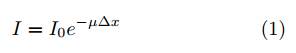
Fig. 5 shows one application using radar particle tracking. A metallic sphere is used as the tracer to measure the drag force exerted by the surrounding particles. Due to the opacity of the sample, it is necessary to have a non-invasive 3D tracking approach to explore what happens within the granular sample. A continuous wave radar system (¹⁷) was used to fulfill the task. Although moving target indicator (MTI) radar is typically used in scenarios at large length scales (e.g., assist aircraft landing or taking-off), it is possible downsize it to the laboratory scale to trace centimeter or even smaller sized particles (51). In this specific case, the above challenges can be resolved by means of (i) selecting tracer and surrounding particles such that they have very different dielectric constants to ensure good SNR. More specifically, porous particles can be used to ensure good penetration of EM waves. (ii) Calibration is performed with tracers moving in a well defined circular trajectory. Typically, multiple runs of the calibration process are needed to ensure an accurate determination of calibration parameters such as the positions and orientations of individual antennae. In addition, polarization of the antennae should be adjusted during the calibration process. (iii) Depending on specific applications, we may choose continuous wave (CW) radar for extremely fast dynamics, or switch to FMCW mode for tracking multiple particles.

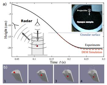
Figure 5 (a) The trajectory of a spherical metallic tracer impacting onto opaque Styrofoam particles (see upper right inset for a snapshot of the sample) obtained with a radar setup (see lower left inset for a schematic of the setup) together with the result from numerical simulations. Gray shaded region corresponds to the uncertainty of the trajectory based on multiple runs of experiments. (b) Projectile (red) impact on a granular material composed of spherical particles (silver). Data extracted from the DEM simulation of a corresponding experiment (¹⁷). 

In both SNR enhancement and IQ mismatch correction, how to effectively and robustly smooth raw data collected at different sampling rates and uncertainty levels requires substantial care. Given the fact that the trajectories of tracers are unknown, fitting the raw data with pre-defined trajectories and parameter settings won’t help in extracting relevant information. Thus, non-parametric algorithms such as moving average filtering, smoothing splines or local regression are feasible approaches. In particular, Gaussian Process Regression (GPR) has emerged as a suitable method with the ability to handle data with complicated patterns. As a machine learning (ML) algorithm, it trains a model with the collected data for prediction (100). The advantage is that it does not rely on a pre-defined analytic expression, but on the Gaussian distribution of ordinate values at different abscissa data points. Nevertheless, one needs to carefully evaluate computational cost spent in training the model while implementing GPR. Previous investigations (100) show that GPR has a space complexity of N _i ³ and time complexity of N _i ² with N _i the number of data points. For the example described above, N may easily reach 10⁵, therefore an appropriate choice of the kernel function and sampling rate for data smoothing to balance efficiency and accuracy is necessary.

For the projectile impacting example described above, an accurate determination of the tracer trajectory does not necessarily mean that we are ready to explore the collective dynamics of surrounding particles. In this regard, synergy with numerical simulations becomes essential. As shown in Fig. 5(a), direct simulations of the experimental condition provide an opportunity to explore the dynamics of all relevant particles during impact. On the one hand, experimental data can be used to calibrate DEM simulations (see, e.g., Fig. 5(b)). On the other hand, DEM simulations provide indispensable insight into the experimental results, with great detail. A calibrated numerical model enables further analysis of mechanical response of the system from a ‘microscopic’ perspective.

Although radar tracking is relatively new in the family of ‘imaging’ particles, it has the potential to develop as a compact, cost-effective, energy efficient, and accurate particle tracking approach because of recent advances in radar-on-chip (RoC) technologies. Nowadays, RoC has become widely used in applications such as autonomous driving and gesture recognition (97). Modern onchip radar effectively embeds transmission antennae (Tx-Ant.), receiving antennae (Rx-Ant), oscillators, amplifiers and other components into a single micro-chip with surface area smaller than 7×7mm². Together with micro-controller and other peripheral components, it it possible to embed the whole system into a hand-held device, as Fig. 4(a) shows. Depending on the bandwidth it operates, commercial models of on-chip radar are capable of measuring a centimeter sized tracer at a spatial resolution of centimeter scale within a range of 10 ∼ 20 meters. The working distance arises from the damping of EM waves in the sample as well as from the capability for the target to scatter EM waves (characterized by radar cross-section), as indicated by the Radar equation (96). As such, the minimal size of the target and working range of the radar depend on the power, operation wavelength and cross-section of the tracer, as well as the surrounding environment. For on-chip radar with limited power consumption, further considerations are needed to implement it in particle tracking. The wavelength of commercially available on-chip radar systems is on the order of millimeters, thus it theoretically possible to track particles of millimeter size or even smaller. Note that in a previous investigation (51), tracking a tracer of 5mm in diameter using EM wave of wavelength 3cm was achieved.

iii . ‘Smart’ particles

Apart from the methodologies described above, ‘smart’ particles with embedded sensors (see Fig. 2(c)) have arisen as an alternative for probing the interior of a granular sample. Along with the development of MEMS (micro-electromechanical systems) technologies, sensors such as IMU (inertial measurement units) capable of measuring angular velocity, acceleration, magnetic fields, and other properties can be encapsulated in a microchip with a typical size of a few millimeters for convenient integration into the peripheral circuit with a micro-controller. Since the pioneer use of accelerometers in tracing projectile motion inside a granular medium (101), there have been substantial progresses in developing more robust and accurate tracking algorithms for the detection of tracer position and velocity in both translation and rotational degrees of freedoms by means of sensor fusion (see, e.g., (102)). As IMU sensors become more and more widely used in consumer products, they become more compact, easier for system integration and data transmission, and more readily available. This progress sheds light on further development of ‘smart’ tracers for comprehensive tasks with broader applications in industries (see e.g., (103)). This technique is particularly useful in conditions where conventional 3D imaging techniques cannot be easily implemented, e.g., in microgravity experiments or in exploring inaccessible regions where space, power, and safety limitations arise. In those scenarios, the possibility of having ‘smart’ particles capable of ‘tracing’ themselves and their surroundings, as well as sending data via wireless communications extends our ability to ‘see’ through particulate materials.

In practice, there are three main challenges in accurately determining the position of the ‘smart’ tracers:

1. Coordinate transformation: Raw data collected from IMU sensors include angular velocities and accelerations measured in sensor coordinate. Step-by-step coordinate transformation into a fixed laboratory frame is necessary as the moving target may rotate while traveling. For a successful reconstruction, accurate synchronization of accelerometer and gyroscope during the sampling process, removing drifting of the sensor output, as well as an appropriate selection of sampling rate need to be carefully considered (102).

2. Cumulative error: After obtaining acceleration in a fixed coordination system, integration is needed to obtain velocity and position of the tracer. During this process, error arising from background noise, drift of the raw signal, as well as uncertainty from coordinate transformation, will accumulate. It is recommended to use techniques such as a combination of forward and backward integration to reduce accumulated error (102).

3. Calibration: While talking about particle tracking, we typically consider measuring geometrical center or center of mass. In either case, the goal is to obtain the trajectory of a fixed point of the tracer particle. Nevertheless, the embedded sensors are not necessarily at the desirable location and different sensors might be located at different locations. Consequently, the acceleration measured might include, e.g., centrifugal acceleration components. Thus, calibration for sensor position is needed for an accurate reconstruction of the tracer trajectory.

For more specific challenges associated with individual steps described above, interested readers may refer to a recent article (102). In the future, the development of sensing technology allows more information, such as local humidity and temperature, force applied on the surface, magnetic field, to be collected as ‘smart’ particles going through the sample. It is possible to design ‘smart’ rotors that can effectively explore the sample by themselves actively, in addition to the swarmed tracers described above (103). Moreover, ‘smart’ tracer network with communications and data sharing among them provides the opportunity for the implementation of data analytical approaches to enhance the ‘smartness’ of the sensing network. In short, if power consumption of the sensing units is further reduced, this technology has a great potential to develop itself into a powerful tool to explore particulate materials from an ‘insider’ perspective.