TRABAJOS DE INVESTIGACIÓN

Co-seismic deformation of the 2010 Maule, Chile earthquake: validating a least squares collocation interpolation

Deformación co-sísmica del terremoto de Maule, Chile de 2010: validación de una interpolación por colocación por mínimos cuadrados

 

Gómez,D.D.^1,2, Smalley, R.¹, Langston, C.A.¹, Piñón, D.A.^3,2, Cimbaro, S.R.², Bevis, M.⁴, Kendrick E.⁴, Barón, J.⁵, Báez, J.C.⁶ and Parra, H.⁷

¹ Center for Earthquake Research and Information, The University of Memphis, USA - 3890 Central Ave, Memphis, TN 38152, United States of America.
² Instituto Geográfico Nacional, Argentina - Avda. Cabildo 381 C1426 - AAD C.A.B.A. República Argentina.
³ RMIT University, Australia – 402 Swanston St, Melbourne, Victoria, 3000 Australia.
⁴ The Ohio State University - 281 W. Lane Ave., Columbus, Ohio 43210, United States of America.
⁵ Universidad Nacional de Cuyo, Argentina. - Centro Universitario, Ciudad de Mendoza, Provincia de Mendoza, República Argentina.
⁶ Universidad de Concepción, Chile. Víctor Lamas 1290, Concepción, Octava Región, Chile.
⁷ Instituto Geográfico Militar, Chile. Santa Isabel 1640 Santiago de Chile, Chile.
E-mail: ddgomez@memphis.edu

---

ABSTRACT

Least squares collocation (LSC) has been successfully applied to develop the Velocity Model for SIRGAS (VEMOS) (Drewes and Heidbach, 2012) used to predict the velocities in the Geocentric Reference System for the Americas (Sistema de Referencia Geocéntrico para las Américas, SIRGAS) GNSS reference frame. After the 2010 (Mw 8.8) Maule, Chile earthquake, the co-seismic and ongoing post-seismic deformation changed both the coordinates and velocities of geodetic benchmarks and continuous operating GPS reference stations (CORS) within the region affected (latitude -28 to -40). This deformation made VEMOS invalid for the estimation of velocities in the reference frame. To correctly obtain coordinates in the pre-seismic frame using post-seismic coordinates, it is necessary to estimate the deformation produced by the earthquake, both co- and post-seismic. Since neither the Argentine nor the Chilean CORS GPS networks are sufficiently dense to directly determine the deformation at arbitrary locations (by using the closest station), a densification of the observations of the deformation field using LSC was recently proposed. In this paper, we used a finite element model (FEM) to simulate the co-seismic deformation of the 2010 Maule earthquake. The FEM was then used to test the LSC of the co-seismic deformation field. We found that LSC cannot be used to correctly predict the behavior of the deformation in the near field due to the complexity of the elastic response of the earth’s crust. Nevertheless, the method correctly interpolates the far field deformation. As an alternative to the LSC method, the authors propose to use a finite element geophysical model that allows for a correct approximation of the co-seismic deformation, both in the near and far fields.

Keywords: Least squares collocation; Earthquake deformation interpolation; GPS; Finite element model.

RESUMEN

La colocación por mínimos cuadrados (CMC) ha sido aplicada con éxito para el desarrollo del Modelo de Velocidades para América del Sur y El Caribe (VEMOS) (Drewes y Heidbach, 2012) para predecir las velocidades del marco de referencia GNSS Sistema de Referencia Geocéntrico para las Américas (SIRGAS). Luego del sismo de Maule (Mw 8.8), Chile en 2010, la deformación co- y post-sísmica ha modificado tanto la velocidad como la posición de las marcas geodésicas y estaciones GPS permanentes dentro del área afectada (latitud -28 a -40). Esta deformación ha generado que las estimaciones brindadas por VEMOS sean inválidas. Para la correcta obtención de coordenadas en el marco pre-sísmico utilizando coordenadas post-sísmicas, es necesario contar con una estimación de la deformación provocada por el terremoto, tanto co- y post-sísmicas. Dado que las redes de estaciones GPS permanentes de Argentina y Chile no son lo suficientemente densas para la correcta determinación directa de la deformación (mediante la utilización de la estación más próxima), se ha propuesto la utilización del método de CMC para densificar y predecir los desplazamientos co- y post-sísmicos. En esta publicación, se utilizó un modelo de elementos finitos para simular el sismo de Maule de 2010. Dicho modelo fue luego utilizado para corroborar los resultados de la interpolación por CMC del campo de deformación co-sísmico. Hemos hallado que la predicción por CMC no logra predecir adecuadamente las observaciones en el campo cercano al epicentro, debido a la compleja respuesta elástica de la corteza terrestre. Sin embargo, el método interpola correctamente la deformación del campo lejano. Como alternativa al método propuesto, los autores propondrán la utilización de un modelo geofísico de elementos finitos que permite una correcta aproximación de la deformación co-sísmica, tanto en el campo cercano, como en el campo lejano.

Palabras claves: Colocación por mínimos cuadrados; Interpolación de deformación sísmica; GPS; Modelo de elementos finitos.

---

 

INTRODUCTION

Mathematical representations of observational data are comprised of deterministic and stochastic models. A deterministic model is defined by a functional relation between the observed data and the model parameters describing the physical characteristics of the phenomenon under study. In inverse theory, this model is usually presented in the form of a matrix multiplication as Ax=L, where A represents the functional relation (also known as the design matrix), x is a vector of model parameters and L is the observation vector (Sevilla, 1987).
The stochastic model is the mathematical representation of the random behavior of the phenomenon, which can be described in terms of a probability density distribution. The statistical expectation of the variables is given by means of the covariance matrices, which describes the random behavior of the data and model parameters (Moritz, 1972). During least squares adjustment, the stochastic model is often used to weight the data by multiplying the inverse of the covariance matrix, , with the a priori unitary variance to obtain the socalled weighting matrix. If we have independent direct observations, the covariance matrix will only have elements on the diagonal that correspond to the expected variance of the observations, thus representing their probability distribution. This implies that we at least know the mean (assumed to be zero) and variance of the probability distribution that governs the random behavior of the observations. When the physical laws that govern the phenomena under study are unknown or their expressions are too complicated to be derived, we can consider the observations to be random variables of a particular probability density distribution with their mean located at the observation value. In this case, we can fit the deterministic part of the observed variable with a convenient function (such as a polynomial) that has no physical meaning (Vieira et al., 2009). To apply geostatistical tools such as least squares collocation (LSC), it is required that the misfit between the data and the function describing the deterministic part of the problem produces residuals with a probability distribution that has a mean statistically equal to zero. By analyzing the statistical behavior of a variable under study, i.e. describing its stochastic model, the LSC method can be used to obtain spatial or temporal predictions (interpolations) of the variable of interest. This stochastic model description can be done analytically to find the exact expression of the so-called covariance function. In most cases, however, this analytical form may be very complicated and hard to derive. Nevertheless, Moritz (1978) showed that although the statistical interpretation of the covariance function provides a solution with a minimum root mean square (RMS) interpolation error, any expression can be used to describe the covariance of the data, as long as the resulting covariance matrices are symmetric and positive definite. This is generally done by fitting a suitable expression to the empirical covariance data, which will provide a simple and optimal way to obtain a result that is within a certain tolerance of the minimum RMS solution (Moritz, 1978).
This procedure has been successfully applied in geodesy for gravity and other variables such as the velocity field of the Caribbean and South American plates in the Sistema de Referencia Geocéntrico para las Américas (SIRGAS) 2000 reference frame (Drewes and Heidbach, 2012). Recently, the application of LSC to predict the elastic deformation of the 2010 Maule earthquake was proposed by Drewes and Sánchez (2013) during the SIRGAS meeting in Panamá City. By analyzing the empirical covariance data of the available GPS sites during the time of the earthquake, they have constructed a one degree grid in latitude and longitude of predicted co-seismic deformation to interpolate the displacements that relate the pre-seismic reference frame with the post-seismic one. By fitting the ongoing post-seismic deformation (using the same technique), they have proposed a practical way to "connect" these two reference frames. As it was previously discussed, the LSC method has proved to be a reliable technique to interpolate gravity observations, since the gravity equipotential is oftentimes a continuous and smooth surface. However, Darbeheshti and Featherstone (2009) showed that in some cases, where the gravity field shows sharper changes across faults and other geologic features, non-stationary LSC must be used in order to better interpolate the equipotential surface. Because the deformation of an earthquake can also show abrupt changes in the near field (especially across fault lines), which might not be correctly sampled due to the lack of observations, a deeper analysis of the problem must be conducted in order to understand the capabilities and limitations of this interpolation method.
To better test the proposed application of LSC to elastic deformation produced by the Maule earthquake, we have simulated the co-seismic deformation by means of a finite element model (FEM) using a finite element code for dynamic and quasistatic simulations of crustal deformation called Pylith (Aagaard et al., 2013). This simulation provides a convenient way to solve a forward LSC problem, by knowing a priori the magnitude of the deformation. These tests have revealed that the application of the LSC method to deformation data cannot correctly interpolate the deformation in the near field, using the available GPS dataset. Nevertheless, the far field interpolation results are in good agreement with the synthetic deformation values from the FEM. These results suggest that it might be necessary to consider other LSC approaches such as non-stationary covariance functions, although this will not mitigate the effect of the lack of observations in some regions where the FEM shows a complex elastic response.

THE LEAST SQUARES COLLOCATION METHOD

Using both deterministic and stochastic components, the observation of a physical quantity may be expressed as:

where z is the observed variable, A is the design matrix, x is the model parameters vector, Ax represents the deterministic component, s is the stochastic component signal vector, and n is the measurement noise. Assuming that the noise measurement in (1) is uncorrelated between independent observations, the stochastic signal s and noise n may be obtained by evaluating the following expression

The left hand side of equation (2) contains the residuals that are not represented by the deterministic model. If the deterministic model has no physical meaning, i.e. the design matrix A is an arbitrary fitting function that produces residuals with a mean that is statistically equal to zero, obtaining the residuals s+n can be interpreted as a detrending of the observations. The necessity of detrending the data to apply LSC will be discussed later in this section. Quantity s (also known as the stochastic signal) can be modeled using a stochastic model defined by the covariance matrix C with elements

where E(si, sj) is the mathematical expectation operator, Cij is the ij element of the covariance matrix C and si,sj are the ij elements of the stochastic signal s. Since the noise term n is uncorrelated for independent measurements, the measurement noise matrix can be written as

where σ2 is the variance of the observations. We are using a uniform variance because we are assuming the measurements are obtained from a single observational method (e.g. GPS). The covariance matrix will then be the sum of (3) and (4) which yields:

As previously discussed, the covariance of the measurement errors is equal to zero but the covariance of the stochastic signal is non-zero, allowing us to separate them and model the stochastic signal. Obtaining an exact mathematical expectation expression for C in (5) is oftentimes a difficult task. To avoid these complications, a function can be fit to the covariance data to obtain the so-called covariance function (Moritz, 1978). This function must satisfy the conditions that the resulting covariance matrices are symmetric and positive definite. To obtain the covariance data, observation residuals from equation (2) have to be grouped into "bins" according to their pair distance. Then, the covariance for each distance dj will be the average of the covariance of the j’s bin, which contains Nj pairs and can be calculated as:

where is the residual from equation (2). A function that describes the general characteristics of the covariance data as a function of distance must be used to fit the empirical covariance data points obtained from (6). The most common types of functions used to fit covariance data are the Cauchy (Moritz, 1980):

and Gaussian expressions (Kearsley, 1977):

for stationary cases, where C0 is the a priori variance, d is the distance and r1,r2 are the correlation lengths. Equivalent non-stationary expressions for (7) and (8) are presented in Darbeheshti and Featherstone (2009). Detrending the data using equation (2) is a necessary step before finding the covariance function. In two dimensional data sets (scalar fields) with trends, the expectation value of the field changes as a function of position. The so-called intrinsic hypothesis states that the expectation value of the scalar should not be a function of position (Ligas and Kulczycki 2010; Vieira et al., 2009), thus the detrending of the data is a necessary step to satisfy the intrinsic hypothesis. To verify that the data set satisfies this hypothesis, one can plot the semi-variogram of the variable under study. When the semi-variogram has a clearly defined and stable plateau or sill at the value of the a priori variance, the intrinsic hypothesis is satisfied and therefore, geostatistical analysis such as kriging or LSC can be applied to the data (Vieira et al., 2009). Once the covariance function has been estimated, the values at unmeasured points can be "predicted" using LSC:

 

where z is the observation vector, ss C has been already defined and zs C is the covariance matrix of the predicted points. The zs C matrix is calculated using the same covariance function as for ss C , since the distances between observation and prediction points are known. After finding the stochastic signal sp, the complete observation estimate can be calculated by adding the detrending function or deterministic model back. So, the complete predicted data can be found using the following expression:

If the data has no trend, then the result from equation (9) provides the desired prediction. The LSC method has been successfully applied to a number of problems, such as topographic interpolation, gravity measurements and geodetic reference frame velocities. Its application to other fields, such as elastic deformation, can be done only after validating that the intrinsic hypothesis is satisfied. For the elastic deformation case, this validation might be a difficult task to perform, as the available data to perform semi-variogram plots can be very limited. Moreover, since the deformation signal can have a very complicated spatial structure in unsampled regions, the direct use of LSC might provide "visually" good results that do not match the actual deformation field. To test and validate the procedure, we have obtained synthetic data to test the LSC application to elastic deformation.

SYNTHETIC DATA FOR FORWARD VALIDATION

In order to obtain synthetic data to test the application of LSC to elastic deformation data, we have used the finite element model (FEM) code Pylith. The finite element method is a numerical technique for finding approximate solutions for governing differential equations. Pylith is a numerical approach to solve dynamic and quasistatic elasticity problems. The construction of a FEM starts by defining a mesh of nodes to which the finite element method will be applied. The complexity of the model geometry and boundary conditions vary from problem to problem. Since the purpose of our FEM is to obtain an approximate co-seismic deformation field to use in our synthetic LSC test, we only include in the model first order characteristics that have the greatest impact on co-seismic deformation.
As the region under consideration extends from Chile to eastern Argentina, a flat earth or half-space model is inappropriate to model the deformation field and therefore, we have used a layered spherical FEM mesh. Layer thickness and elastic properties are taken from the Preliminary Earth Model (PREM) (Dziewonski and Anderson, 1981). One of several advantages of using a spherical FEM mesh is that there is no necessity to define free slip boundary conditions, as deformation in a sphere is self constrained, since the nodes that form the FEM mesh form a closed surface. After the FEM mesh geometry is defined, a fault model must be used to simulate the slip produced by the earthquake. Several finite fault models are available based on inversion of InSAR data, GPS or both (Tong et al., 2010; Pollitz et al., 2011; Lorito et al., 2011; Moreno et al., 2012). Because of the particular characteristics of our FEM model, we have inverted our own finite fault model using GPS data only. The input data to produce the finite fault slip model was a combination of the co-seismic displacement solutions obtained from the Central Andes GPS Project (Pollitz et al., 2011) and the Instituto Geográfico Nacional (IGN). This inversion yields the approximate slip distribution on a predefined fault surface. As our fault surface, we have adopted the USGS South American subduction zone slab model (Hayes et al., 2012). We will not discuss the finite fault inversion process and modeling techniques since they are out of the scope of this paper.
Using the FEM mesh and the finite fault model, we run Pylith to produce two datasets: 1) the co-seismic displacements at the same locations where the continuous GPS (CGPS) stations are located and 2) co-seismic displacements on a 0.5º grid in latitude and longitude where the LSC will be used to interpolate the earthquake’s deformation.
Before continuing to the LSC tests, we will show the similarity of the synthetic data to the real co-seismic deformation. This comparison will validate the use of this synthetic dataset to apply LSC as if this was the observed deformation field. Figure 1 shows the comparison between the observed and the FEM co-seismic deformation field. Misfits between the model and the GPS observations can be observed, in both the near and far field. However, these differences never exceed 25 cm, as shown by Figure 2. Taking into account previous simulation residuals (Tong et al., 2010; Pollitz et al., 2011; Lorito et al., 2011; Moreno et al., 2012), the directions of the displacements are in very good agreement with the directions reported by the GPS observations (except for a few points), showing that the model represents the crustal elastic response of the 2010 Maule earthquake well. The misfits are probably due to a combination of the roughness of the mesh and the simplicity of the finite fault model. Since the objective of this paper is to test the LSC of elastic deformation, we conclude that the obtained synthetic dataset is adequate to run our tests.

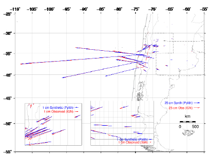
Figure 1: Comparison between observed and FEM co-seismic deformation using GPS solutions provided by the Central Andes GPS Project (Pollitz et al., 2011) and Instituto Geográfico Nacional, Argentina. Blue arrows: modeled displacements; red arrows: observed displacements; red dashed polygon: rupture zone defined by aftershocks.
Figura 1: Comparación entre la deformación co-sísmica observada utilizando las soluciones proporcionadas por el Central Andes GPS Project (Pollitz et al., 2011) y el Instituto Geográfico Nacional, Argentina y la deformación calculada utilizando el MEF. Flechas azules: desplazamientos modelados; flechas rojas: desplazamientos observados; polígono rojo línea de trazos: zona de ruptura definida por las réplicas del terremoto de Maule.

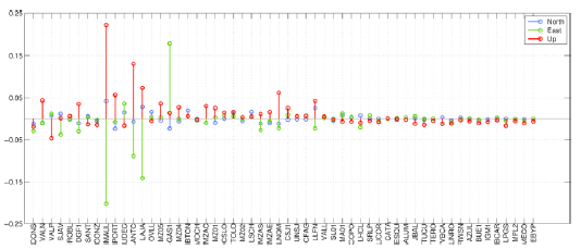
Figure 2: Station list, ordered by increasing distance from the rupture zone, with differences between model and GPS observations for north, east and up components. Only six stations exceed the 5 cm limit, all of them in the near field. These differences are most likely due to model geometry and slip inversion simplifications.
Figura 2: Diferencias entre modelo y observaciones GPS por estación, ordenadas según distancia ascendente a la zona de ruptura, para las componentes norte, este y arriba. Solo 5 estaciones exceden el límite de 5 cm, todas en el campo cercano. Estas diferencias son probablemente debido a las simplificaciones de la geometría del modelo e inversión de parámetros del desplazamiento en la falla.

ELASTIC DEFORMATION SEMI-VARIOGRAM

We have produced semi-variogram plots of the elastic deformation as in Vieira et al., (2009) to investigate if the data satisfy the intrinsic hypothesis, which can be verified by the presence of a plateau or sill in the semi-variogram plot. Unlike the empirical covariance function, which describes the similarity of the data as a function of distance, the semi-variogram provides a measure of the dissimilarity between pairs of observations at a certain distance range (Ligas and Kulczycki, 2010).
The first assumption required to apply the LSC method (with a stationary covariance function) is that the earthquake’s deformation data describes a stationary process. This means that the selected covariance function that describes the stochastic behavior of the data is the same for the entire domain. Although the observed elastic deformation data does not satisfy this assumption, since the deformation field does not have a mean equal to zero (as seen on Figure 1), we can assume an approximate stationary covariance function after detrending the data.
We followed the procedure of Vieira et al., (2009) to obtain the lowest degree detrending polynomial that produces a sill in the semi-variogram plot. Vieira et al., (2009), however, does not discuss the maximum degree for the detrending polynomial, which has to take into account the number of available data points. If the degree of the polynomial is too high and the data points are few, we can obtain spurious oscillations and edge effects due to a badly constrained inversion of the polynomial parameters. From this analysis, we have found that the maximum polynomial degree allowed by the FEM grid is six while the maximum degree for the synthetic GPS solution (that of the FEM at the GPS sites) is only two. The consequences of detrending the data with these two different polynomials will be discussed later.
Figure 3 (left) shows the semi-variogram plot (see data sources section) of the east component co-seismic deformation for the FEM grid (blue circles), the detrended data semi-variogram (green circles) and the semivariogram model (red line). We will only present the results for the east component, since most of the deformation was east-west, however, this procedure was also applied to the north-south component as well. We assumed the following Gaussian model:

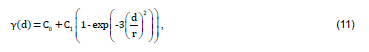
where C0, C1 are the a priori variance and covariance (sill), d is the distance between point pairs and r is the correlation length (Vieira et al., 2009).

Figure 3: left, semi-variogram of the whole deformation field (0.5º by 0.5º grid). Blue circles: deformation without detrending; green circles: detrended deformation; red line: Gaussian semi-variogram model. Right, semi-variogram of the deformation field sampled at the CGPS stations.
Figura 3: izquiera, semi-variograma del campo de deformación completo (grilla de 0.5º por 0.5º). Círculos azules: deformación sin eliminar la componente sistemática; círculos verdes: deformación sin componente sistemática; línea roja: modelo de semivariograma Gaussiano. Derecha, semi-variograma de campo de deformación utilizando sólo la información provista por las estaciones GPS permanentes.

From Figure 3 (left), we observe that the semi-variogram presents an approximate plateau or sill that suggests that the deformation field describes a stationary process. Therefore, after detrending the data using the lowest degree polynomial that produces a sill (two variable, degree five), LSC can be applied using a unique covariance function to describe the stochastic behavior of the deformation field. If we plot the semi-variogram using only the available GPS data (i.e. using only the observations at the CGPS stations) the semi-variogram does not present a clear sill (Figure 3, right). This behavior can be explained by the low number of CGPS observations. Because the maximum polynomial degree that this dataset allows is two, we cannot increase the degree of the polynomial, which would allow the detrending function to produce a semi-variogram with a sill, as in Figure 3, left.
Because less data points are available when using the CGPS observations, the degree of the polynomial has to be low, as discussed earlier. Degree two, however, is not enough to correctly detrend the deformation field (due to the roughness of the co-seismic displacements) and therefore, the semi-variogram does not show a clear sill. When more data points are added to the polynomial fit (as in Figure 3, left), we can increase the polynomial degree and the detrending procedure correctly removes the trend, producing a sill in the semi-variogram. This result suggests that a minimum number of observations exists for which the detrending procedure produces a dataset to which LSC can be applied (Gómez et al., 2014). However, only a limited number of GPS stations were available at the time of the earthquake. Although other datasets could be added such as campaign observations and nonpublicly available GPS solutions, at this time we have only used the currently available data (see the acknowledgements section). Darbeheshti and Featherstone (2009) showed that when the stochastic behavior of the variable under study cannot be described using a stationary covariance function, either a non-stationary covariance function or a partitioned domain can be used to apply LSC. Following Darbeheshti and Featherstone (2009), and to avoid discontinuities in our interpolated deformation field, we have partitioned the domain in triangular sections to apply a stationary covariance function using the data from the nearby locations of the sub-domain. Using this partitioned domain, we applied LSC to obtain an interpolated deformation field that we compared against the FEM to validate our results.

RESULTS

We proceeded to apply LSC to the deformation field to produce an interpolated field on a 0.5º grid in latitude and longitude. In order to reduce the non-stationary characteristics of the elastic deformation field, we have partitioned the domain into sub-domains defined by triangles that enclose similar deformation observations. One covariance function was calculated for each sector using the nearby data. Because bounding triangles share the same observations for two vertices, the boundary patching discussed by Darbeheshti and Featherstone (2009) is less visible than when taking arbitrary rectangular limits. Nevertheless they exist and some smoothing procedure should be applied to remove it, although we did not apply any.
Figure 4 shows the results of the LSC deformation field. The mid to far field LSC interpolation is in good agreement with the FEM results. The good fit of the interpolation to the FEM model can be attributed to the smoothness of the far field data. This smooth behavior of the deformation field yields a subdomain that can be correctly described as a stationary process. Regardless of this good fit, some areas could benefit from extra measurements, although the differences never exceed five to nine millimeters. We should also mention that after analyzing the far field stochastic component of the interpolation, calculated using equation (9), we found that the deformation field was almost completely modeled using the detrending polynomial. As a result, the residual from equation (2) was very small and the stochastic signal obtained with the LSC method had a very low influence on the final solution, obtained from equation (10). In the near field, however, it can be seen that the LSC produced outliers of up to 1.5 meters. These results are in agreement with the semi-variogram obtained during the previous section, which revealed that with the number of available observations, the dataset trend cannot be correctly removed. Moreover, partitioning the domain introduces an important limitation. Because there are fewer data points to fit the polynomial function (since we only use the data inside the partitioned domain), we cannot use a high degree polynomial to remove the trend. If short wavelength deformation exists in the subdomian that cannot be absorbed by the lower degree polynomial, the detrended dataset will not satisfy the intrinsic hypothesis.

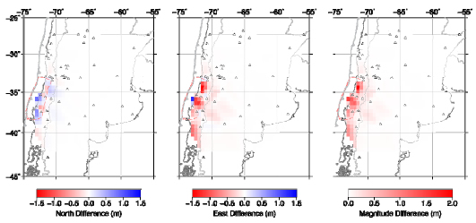
Figure 4: differences between LSC and synthetic co-seismic deformation. Left: North difference; middle: east difference; right: total (magnitude) difference. Triangles: GPS stations used to apply LSC.
Figura 4: diferencias entre LSC y la deformación co-sísmica sintética. Izquierda: diferencia en componente norte; centro: diferencia en componente este; derecha: diferencia total (magnitud). Triángulos: estaciones GPS utilizadas para aplicar LSC.

In the northern and southern edges of the rupture zone (marked in Figure 4 with a red dashed line), some of the interpolated points are highly influenced by the lack of observations in their neighborhood. In these regions, due to the edge effects of the fault rupture, the behavior of the deformation changes very rapidly when crossing outside the rupture zone boundary. The same effect can also be observed in the central section of the rupture zone, as this region also presents rapid changes in deformation vector orientation. This observation suggests that by incorporating more measurements to the LSC, the near field interpolation could be improved. However, these observations might not be available or could be highly influenced by post-seismic deformation. Since the postseismic deformation produced by the earthquake affects the velocity of the GPS stations, obtaining a direct measurement of the co-seismic jump (e.g. from campaign stations observations) might provide an unreliable value that will affect the result of the interpolation. Other options, such as using InSAR data could also be used to increase the number of observations, although they will also be affected by the post-seismic deformation.

DISCUSSION AND CONCLUSIONS

The application of LSC to predict the elastic deformation of the 2010 Maule earthquake was proposed by Drewes and Sánchez (2013), where they showed some results of the interpolation process. To better test the proposed application of LSC, we produced synthetic observations for the earthquake using a FEM. These observations allowed us to analyze and quantify the results of the LSC method of elastic deformation data. The semi-variogram plot of synthetic data showed that when using the available number of CGPS stations (Figure 3, right), the semi-variogram does not clearly show a sill and therefore, the intrinsic hypothesis is not satisfied, resulting in inaccurate interpolations, especially in the near field. This shortcoming can be resolved by either using more observations (since we showed that the semi-variogram of the whole deformation field presents a more stable sill) or a partitioned domain to estimate individual covariance functions. A third option that we did not investigate is the application of non-stationary covariance functions as in Darbeheshti and Featherstone (2009).
Although obtaining more observations is the best option, such observations might not exist, or might not be sufficiently accurate for geodetic and geophysical applications. Campaign data obtained a few months after the main event, for example, will be affected by post-seismic deformation. We could resolve this shortcoming by estimating the ongoing post-seismic deformation to predict the coordinates at the epoch immediately after the earthquake, although this procedure introduces an undetermined uncertainty. We note, however, that the postseismic effect in campaign data (and InSAR) could be negligible for the purposes of creating an interpolated deformation field using LSC, depending on the intended application of such interpolation. At this time, instead of adding more observations, we have partitioned the domain into triangular sections of similar deformation to obtain individual covariance functions of these subdomains. Partitioning the domain, however, introduces an important limitation. Because there are fewer data points to fit the polynomial function (since we only use the data inside the subdomains), we cannot use a high degree polynomial to remove the trend. If there is a significant deformation change in the subdomain that cannot be absorbed by the lower degree polynomial, the detrended dataset will not satisfy the intrinsic hypothesis. An alternative that we tested was to detrend the whole domain followed by partitioning. This option does not provide good results, since the covariance function should be estimated using the entire detrended domain (not just a portion of the detrended domain) to guarantee that the intrinsic hypothesis is satisfied. We proceeded to interpolate the deformation field using the proposed partitioned domain. The far field predictions show overall good agreement with the FEM data. In the near field, nonetheless, collocation produces large outliers at the edges of the rupture zone (of ~1.5 m). The rapid change of the deformation field is characteristic of thrust fault earthquakes such as the 2010 Maule event, which prevents the LSC method from correctly interpolating the deformation field with the available GPS observations. Moreover, a smoothing effect in the near field was observed after applying LSC, which is probably further evidence for a lack of observations.
A better partitioning of the near field domain, the use of non-stationary covariance function and the addition of extra observations could improve the results. Nevertheless, the far field collocation showed that the detrending polynomial can "absorb" almost all of the deformation, leaving a very small residual for the stochastic component to model. This suggests that, if the necessary observations were added during the near field collocation procedure, the elastic behavior will be smooth enough between samples so that other interpolation techniques can be applied to the data. Based on the results presented here, we found that LSC is not an appropriate tool to "predict" elastic deformation using the available dataset. We have shown that more observations are needed in order to obtain a dataset that satisfies the intrinsic hypothesis. We also note that the complexity of the deformation field can be reproduced by a physical representation of the problem, using the equations of elasticity.
To provide observations of the co-seismic deformation between CGPS stations, we propose using a FEM such as that used to obtain the synthetic data presented here. Even with a very rough model, we showed that the FEM produced a deformation field that is in very good agreement with the CGPS observations. By using a better mesh and a more complex finite fault model, we hope to obtain a more accurate representation of the near and far fields. The development of such model is under study and will be presented in the near future.

Acknowledgements

We would like to thank Benjamin Brooks and James Foster for providing additional datasets that were used for this work. We would like to thank Wolfgang Schwanghart for providing his semi-variogram code (see Data sources section). The authors would like to thank two anonymous reviewers for their insightful comments and suggestions that have contributed to improve this paper.
This work was supported by the NSF Office of Polar Programs grant Collaborative Research: IPY: POLENETAntarctica: Investigating Links between Geodynamics and Ice Sheets (NSF-ANT-062339 and supplement - 0948103) and the Center for Earthquake Research and Information, University of Memphis.

REFERENCES

1. Aagaard, B.T., Knepley, M.G., Williams, C.A., (2013). A domain decomposition approach to implementing fault slip in finite-element models of quasi-static and dynamic crustal deformation. Journal Geophysical Research Solid Earth, 118: 3059–3079. doi:10.1002/jgrb.50217.

2. Darbeheshti, N., Featherstone, W.E., (2009). Non-stationary covariance function modelling in 2D least-squares collocation. Journal of Geodesy, 83: 495–508. doi:10.1007/s00190-008-0267-0.

3. Drewes, H., (1978). Experiences with least squares collocation as applied to interpolation of geodetic and geophysical quantities, in: Proceedings of Symposium on Mathematical Geophysics, Caracas.         [ Links ]

4. Drewes, H., Heidbach, O., (2012). The 2009 Horizontal Velocity Field for South America and the Caribbean, in: Kenyon, S., Pacino, M.C., Marti, U. (Eds.), Geodesy for Planet Earth. Springer Berlin Heidelberg, Berlin, Heidelberg, pp. 657–664.

5. Drewes, H., Sánchez, L., (2013). Modelado de deformaciones sísmicas en el mantenimiento de marcos geodésicos de referencia. Presented at the SIRGAS 2013 Meeting, Instituto Geográfico Nacional Tommy Guardia, Panama City, Panama.         [ Links ]

6. Dziewonski, A.M., Anderson, D.L., (1981). Preliminary reference Earth model. Physical Earth Planet. Inter. 25: 297– 356.

7. Gómez, D., Smalley, R., Piñón, D., Cimbaro, S., (2014). Colocación por mínimos cuadrados de la deformación cosísmica del sismo de Maule, Chile 2010: Estimación de observaciones mínimas. Presented at the XXVII Reunión Científica de la Asociación Argentina de Geofísicos y Geodestas, San Juan, Argentina. doi:10.13140/2.1.4254.9445        [ Links ]

8. Hayes, G.P., Wald, D.J., Johnson, R.L., (2012). Slab1. 0: A three-dimensional model of global subduction zone geometries. Journal Geophysical Research. Solid Earth, 1978–2012, 117.

9. Kearsley, W., (1977). Non-Stationary Estimation in Gravity Prediction Problems. DTIC Document.         [ Links ]

10. Ligas, M., Kulczycki, M., (2010). Simple spatial prediction-least squares prediction, simple kriging, and conditional expectation of normal vector. Geodesy and Cartography. 59: 69–81.

11. Lorito, S., Romano, F., Atzori, S., Tong, X., Avallone, A., McCloskey, J., Cocco, M., Boschi, E., Piatanesi, A., (2011). Limited overlap between the seismic gap and coseismic slip of the great 2010 Chile earthquake. Nature Geosciences. 4: 173–177. doi:10.1038/ngeo1073

12. Moreno, M., Melnick, D., Rosenau, M., Baez, J., Klotz, J., Oncken, O., Tassara, A., Chen, J., Bataille, K., Bevis, M., Socquet, A., Bolte, J., Vigny, C., Brooks, B., Ryder, I., Grund, V., Smalley, B., Carrizo, D., Bartsch, M., Hase, H., (2012). Toward understanding tectonic control on the Mw 8.8 2010 Maule Chile earthquake. Earth Planet. Science Letter. 321-322: 152–165. doi:10.1016/j.epsl.2012.01.006.

13. Moritz, H., (1980). Advanced physical geodesy. Advanced Planet. Geol. 1.         [ Links ]

14. Moritz, H., (1978). Least-squares collocation. Review Geophysics, 16: 421–430.

15. Moritz, H., (1972). Advanced least-squares methods. Department of Geodetic Science, Ohio State University Columbus, USA.         [ Links ]

16. Pollitz, F.F., Brooks, B., Tong, X., Bevis, M.G., Foster, J.H., Bürgmann, R., Smalley, R., Vigny, C., Socquet, A., Ruegg, J.-C., Campos, J., Barrientos, S., Parra, H., Soto, J.C.B., Cimbaro, S., Blanco, M., (2011). Coseismic slip distribution of the February 27, 2010 Mw 8.8 Maule, Chile earthquake: CHILE EARTHQUAKE COSEISMIC SLIP. Geophysical Research Letter, 38, n/a–n/a. doi:10.1029/2011GL047065.

17. Sevilla, M., (1987). Colocación mínimos cuadrados. Publicación Univ Complut. Fac Cienc. Mat Inst Astron. Geod.         [ Links ]

18. Tong, X., Sandwell, D., Luttrell, K., Brooks, B., Bevis, M., Shimada, M., Foster, J., Smalley, R., Parra, H., Báez Soto, J.C., Blanco, M., Kendrick, E., Genrich, J., Caccamise, D.J., (2010). The 2010 Maule, Chile earthquake: Downdip rupture limit revealed by space geodesy: DOWNDIP RUPTURE MAULE, CHILE EARTHQUAKE. Geophysical Research Letter, 37, n/a–n/a. doi:10.1029/2010GL045805.

19. Vieira, S.R., Carvalho, J.R.P. de, Ceddia, M.B., González, A.P., (2009). Detrending non stationary data for geostatistical applications. Bragantia 69: 01–08.

20. Wessel, P., Smith, W.H., (1998). New, improved version of Generic Mapping Tools released. Eos, Transactions American Geophysical Union, 79: 579–579.

DATA SOURCES

Pylith web page: http://geodynamics.org/cig/software/pylith/Semi-variogram code provided by Wolfgang Schwanghart: http://www.mathworks.com/matlabcentral/fileexchange/29025-ordinary-kriging

USGS slab 1.0 model obtained from: http://earthquake.usgs.gov/data/slab/

Maps were made using the Generic Mapping Tools version 5.1.1 (Wessel and Smith, 1998)

Recibido: 15-02-2015
Aceptado: 12-07-2015