ORIGINAL ARTICLE

Response of tomato (Solanum lycopersicum L.) to water consumption, leaf area and yield with respect to the number of stems in the greenhouse

Respuesta del tomate (Solanum lycopersicum L.) al consumo hídrico, área foliar y rendimiento con respecto al número de tallos en invernadero

Cándido Mendoza-Pérez ¹, Carlos Ramírez-Ayala ¹, Waldo Ojeda-Bustamante ², Carlos Trejo ¹, Anselmo López-Ordaz ³, Abel Quevedo-Nolasco ¹, Antonio Martínez-Ruiz ⁴

1 Postgraduate in Hydrosciences. Postgraduate College. Mexico-Texcoco highway. km 36.5. Montecillo. Mexico. C.P. 56230. candido@colpos.mx

2 Mexican Institute of Water Technology. Paseo Cuauhnáhuac No. 8535. Colonia Progreso. Jiutepec. Morelos. Mexico. C.P. 62550.

3 Postgraduate in Botany. Postgraduate College. Mexico-Texcoco.

4 National Institute of Forestry. Agricultural and Livestock Research (INIFAP). San Martinito. C.P. 74100. Puebla. Pue.

Originales: Recepción: 14/04/2018 - Aceptación: 27/08/2018

---

ABSTRACT

The objective of this study was to analyze tomato responses to water requirements (evaluated by means of balance lysimeters), leaf area, yield, quality and its relationship with weather, depending on the number of stems. The work was carried out in a greenhouse under hydroponic conditions. Tezontle (Stuff) was used as a substrate and a drip irrigation system was installed. The experiment consisted of three treatments, with one (T1), two (T2) and three (T3) stems per plant. The daily crop evapotranspiration was 0.30 L m^-2 in the initial stage, up to 4.41, 4.77 and 6.0 L m^-2, in the stage of maximum demand for T1, T2 and T3. The gross volume applied throughout the cycle was 352.2, 388.4 and 434.7 L m^-2 for T1, T2 and T3, with productivities of 49, 41 and 36 kg m³ and yields of 20, 18 and 16 kg m^-2 for T1, T2 and T3. Regarding quality parameters in size, T1 was the best, with 69, 23, 8 and 1% fruits of first, second, third and small fruits per plant respectively. The meteorological variables such as; temperature, wind, relative humidity, vapor pressure deficit and atmospheric water potential determined the consumption of water and nutrients in crops and are variables for irrigation scheduling.

Keywords: Solanum lycopersicum L.; Balance lysimeter; Tezontle; Evapotranspiration; Fruit quality

RESUMEN

El objetivo de este estudio fue analizar las respuestas del jitomate a los requerimientos hídricos (evaluado por medio de lisímetros de balance), área foliar, rendimiento, calidad y su relación con el tiempo atmosférico, en función del número de tallos. El trabajo se realizó en un invernadero en condiciones de hidroponía. Se utilizó tezontle como sustrato y un sistema de riego por goteo. El experimento consistió en tres tratamientos, con uno (T1), dos (T2) y tres (T3) tallos por planta. El consumo por evapotranspiración diaria del cultivo fue 0,30 L m^-2 en la etapa inicial, hasta 4,41, 4,77 y 6,0 L m^-2 en la etapa de máxima demanda para T1, T2 y T3. El volumen bruto aplicado durante todo el ciclo fue 352,2; 388,4 y 434,7 L m^-2 para T1, T2 y T3, con productividades de 49, 41 y 36 kg m³ y rendimientos de 20, 18 y 16 kg m^-2 para T1, T2 y T3. Con relación a los parámetros de calidad en tamaño, el T1 fue mejor, con 69, 23, 8 y 1% frutos de primera, segunda, tercera y frutos pequeños por planta. Las variables meteorológicas como temperatura, viento, humedad relativa, déficit de presión de vapor y potencial hídrico atmosférico determinan el consumo de agua y nutrimentos en los cultivos y son variables para calendarización del riego.

Palabras clave: Solanum lycopersicum L; Lisímetro de balance; Tezontle; Evapotranspiración; Calidad de fruto

---

INTRODUCTION

Tomato crop (Solanum lycopersicum L.) is one of the most consumed vegetables in the world (Chapagain and Wiesman, 2004) and mainly grown under greenhouses. In Europe and the United States, the intensive production system in greenhouses has use undetermined growth habit cultivars and low densities that vary from two to three plants per square meter; where the stems of the plants are often pruned and set a single stem that reaches more than seven meters in length and it is left to harvest 15 or more bunches per plant in a single crop cycle per year (3). This production system in Mexico is relatively new and has generated an impact on the increase in cultivated area, productivity, profitability and quality in recent years.

Production under protected or forced conditions has several advantages over open field production: greater efficiency in the use of water, soil and fertilizers, as well as greater flexibility in the sowing and harvest season according to the market demand.

By having better control over environmental and agronomic variables, greenhouse production is usually better, in quality and quantity than that produced at open field (7, 16, 18, 26).

Irrigation application timing and quantity determine the yield of crops in these systems. In addition, that helps to increase water use efficiency. Thus, a poor coupling of irrigation with water demands of the crop can promote the presence of pests, diseases and physiological disorders (1, 19, 25).

The necessary amount of irrigation should be applied to cover water consumption of the crop by the evapotranspiration (10).

In Mexico, empirical equations have been used for determination of evapotranspiration in protected environments, but it is not known exactly if these values are correlated with the real evapotranspiration, since there is a lack of evapotranspiration data measured over the crop cycle. It is necessary to establish a simple and economical procedure in order to estimate the crop evapotranspiration in protected environments, that can allow adjust such estimation based on meteorological variables (29). The balance method is the most used method to directly estimate the evapotranspiration in which evaporation is measured from bare soil and crop transpiration. Lysimeters are containers with soil generally installed in the field under natural environmental conditions; where water, soil, plant, atmosphere system can be regulated, allowing to measure more accurately. Those lysimeters are used to study environmental effects and to evaluate the estimation methods for water demand of crops (8). That allows calculating the actual evapotranspiration of the crop (ETc) and thus estimating the loss of moisture in the soil, plant, and atmosphere system, which allows scheduling irrigation timing (13).

Greenhouse irrigation is usually applied on drip system with a pre-established interval and timing. This empirical practice does not consider the dynamic conditions in the management, environment and development of the crop. When there is no coupling between irrigation and crop evapotranspiration demands, there are periods of moisture deficit that affect the potential productivity of the crop and the efficient use of water and fertilizers (5).

Development of many organisms is controlled mainly by environmental temperature. Thermal time is an indirect measure of growth and development of plants and insects. These represent the integration of two temperature thresholds, which is define as interval in which an organism is active. Outside this interval, the organism does not show appreciable development or die.

The concept of thermal time resulted from observations indicated: 1) plants do not develop when the ambient temperature is lower than the basal one (Neild and Smith, 1997), 2) the rate of development increases when ambient temperature is higher than the basal one, 3) the varieties of tomatoes require different values of growing degree days.

Knowledge of tomato water demands will allow coupling this demand with the application of irrigation in a timely and efficient manner, and as a result, an increase in the efficiency of fertilizer application, a reduction in contamination, an increase in yield and fruit quality.

Objective

Analyze tomato responses to water requirements (evaluated by means of balance lysimeters), leaf area, yield, quality and its relationship with weather, depending on the number of stems.

MATERIALS AND METHODS

Description of the experiment

The experiment was carried out in a greenhouse at graduate college Montecillo Campus, State of Mexico, (19° 28'05" latitude North and 98° 54'31" longitude West at 2.244 m altitude). In a greenhouse with plastic covers of high-density polyethylene, 75% transmissivity, natural ventilation, and anti-aphid mesh screen equipment. The average temperature recorded during the crop growing cycle was 18.45 °C, 25.0 °C for the hottest month (April) and 9.0 °C for the coldest month (September).

Cultivar “Cid F1 ” seeds were sown on March 5th, transplanted on April 20^th and harvested at the last bunches of fruits on September 20^th, 2015. The plants were maintained at one, two and three stems, and were sprouted on July 8, 2015, when the tenth floral bunches were reached. The arrangement of transplanting consisted of separation of 40 cm between plants and 40 cm between lines in all treatments, using 35 x 35 cm black polyethylene bags with red tezontle (stuff) as substrate, with a crop density of 3 plants m^-2.

Treatments (T) consisted of three management conditions, depending on the number of stems per plant: with one (T1), two (T2) and three (T3) stems per plant, respectively. The area of each treatment was 53 m² with a total area of 159 m². The treatments were distributed in the field under a design in random blocks with arrangement in divided plots with four repetitions whose dimensions were 10 m². The drip irrigation system consisted in a surface irrigation line of 16 mm of diameter, with self-compensating dripper, flow rates of 4 L h^-1, an operating pressure of 68.64 k Pa. The nutrient solution was applied with Steiner solution (27).

The physical properties of five tezontle (volcanic rock) samples were determined. The results were as follows: water holding capacity 1.7 L, bulk density 1.04 g cm^-3, total porosity 40.98%, air capacity 59.44%, field capacity 0.183 cm³ permanent wilting point 0.09 cm³ volumetric water content 0.092 cm³ cm^-3.

Description of variables

Temperature (Ta, oC) and relative humidity (RH, %) were recorded with a data acquisition system, Hobo U12-011 was installed inside the greenhouse at 2 m above the ground. With these variables, the vapor pressure deficit (VPD, k Pa) and atmospheric water potential (Ѱ _w ) were computed from planting to harvest of the tenth bunches. The VPD is a useful variable to express the vapor flow (gradient) in a greenhouse. It also allows knowing the flow of the condensation and the crop transpiration. Besides, it quantifies the proximity of greenhouse air to the saturation.

To estimate the daily degree of development, it was used the (equation 1) that requires the average environmental temperature (17).

ADD= T _a -T _c-min, si T_a < T_c-max

ADD= T _c-max - T _c-min, si T_a ≥ T_c-max

ADD= 0, si T _a ≤ T _c-min

where:

T _a, = the daily air temperature

T _c-max and T_c-min, = minimum and maximum air temperature, the threshold for the tomato growth are 29 and 11 oC (24).

The accumulated values for n days are expressed with:

Where:

i = the number of the day from the initial day, either at planting or the first phenological stage

To measure the evapotranspiration of the crop, control pots with 10 kg of tezontle and water holding capacity of 1.7 L. were used. In each treatment, four replicates of control pots were installed and covered with plastic on the surface to avoid evaporation of water from the substrate. In these pots, a known volume of water was applied at 9:00 a.m, which was allowed to drain for 50 minutes and the drained nutrient solution was measured, and by difference (volume applied and drainage), the evapotranspirated volume was obtained per plant (figure 1).

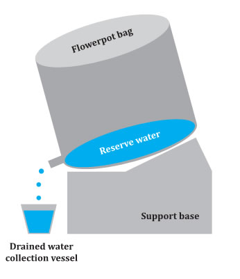
Figure 1. Daily evapotranspiration measurement in control pots in the greenhouse.

Figura 1. Medición de evapotranspiración diaria en macetas control en invernadero.

This procedure was repeated daily at 11:00, 13:00, 15:00 and 17:00 hours with five daily measurements from transplant to harvest of the tenth bunches.

The evapotranspiration during a certain period was the difference between the water supply and the drainage:

ETc = R – D ± Δθ (3)

where:

ETc = crop evapotranspiration

R = the irrigation volume (L)

D = the drainage volume (L)

Δθ = the rate of water content in the substrate (L)

In the absence of rain and other inputs, the irrigation requirements are equal to actual crop evapotranspiration (ETr) described by the following equation.

RR = ETr = transpiration (L) (4)

In addition, pH and EC in the nutrient solution supplied and drained were measured from the pot in order to know the concentration of ions in the solution. In order to adjust the fertilization scheduling to carry out a better control in supplying the nutrient solution.

Relationship between leaf area index and water requirement

In addition, from the measurement of water consumption, the leaf area index was measured in different crop stages to correlate with the water demand of the plant.

In each harvest, quality classification of fruit size was divided into five categories (extra-large, large, medium, small and smallest fruits) based on the Mexican Standard (table 1).

Table 1. Saladette tomato fruits classification (15).

Tabla 1. Clasificación de frutos de jitomate tipo saladette (15).

To determine the significant differences of the evaluated variables, analysis of variance (ANOVA) was conducted along with Tukey mean separation test (P ≤0.05) using MINITAB statistical software.

Water use efficiency (WUE) estimated as the ratio of total yield (kg) and the volume of water applied (m³) as well as yield (R) of the treatments mass produced per unit surface (kg m^-2).

Electric conductivity and pH values managed

The pH values of the nutrient solution were the average of 6.85, and ranged from 6.7 to 7.0; for electrical conductivity (C.E) the average was 1.85 dS m^-1 and varied between 1.1 and 2.6 dS m^-1. The average values for drained solution were 7.6 for pH and 2.89 dS m^-1 for electrical conductivity. These values of electrical conductivity for the drained solution were lower, that recommended for production in greenhouses, whose typical interval is between 2 and 4 dS m^-1.

RESULTS AND DISCUSSIONS

Temperature and relative humidity

At the initial stage of crop, the temperature reported was higher than 22°C, during the hottest months from April to June, and then decreased. In the rainy months from July to September, it decreased until 9°C, and increased the relative humidity up to 90%, due to the rain, cloudy days at the beginning of the cold season where the experiment took place (figure 2, page 93).

Figure 2. Temperature and relative humidity in the greenhouse during the crop cycle.

Figura 2. Temperatura y humedad relativa en el invernadero durante todo el ciclo de cultivo.

The behavior of these two variables were similar to those reported by Jaimez et al. (2005).

Vapor Pressure Deficit (VPD)

Vapor Pressure Deficit (VPD) is an important variable in the crop production, either, in protected conditions or open field. It indicates that when air becomes saturated, the water will condense to form clouds, dew or water films over the leaves. This is the last instance that makes the VPD important for the regulation of water demand. If a film of water keeps on the leaf of the plant, it becomes much more susceptible to putrefaction (20).

The VPD in the stage of vegetative development was 1.7 k Pa. This value could be due to the initial phase of growth, its leaf area was small, so the number of stomata was scarce.

Although the transpiration rate was high, as well as the loss of water vapor inside the greenhouse, this did not reach to satisfy the atmospheric demand. This process involved greater release of water vapor through the stomata of the leaves trying to cover the atmospheric water demand (figure 3, page 94).

Figure 3. Daily vapor pressure deficit (A) and for a day (B) in the greenhouse.

Figura 3. Déficit de presión de vapor diario (A) y durante un día (B) en invernadero.

A high VPD increases the transpiration demand, increases water and nutrient uptake, increasing the photosynthetic activity, in addition, it directly influences the amount of water in plant tissues that is further transferred to the greenhouse air. In the final stage of cultivation, the VPD close to 0.1 kPa was estimated, since the plants decreased the transpiration, because the atmosphere was practically saturated with vapor water.

Therefore, less diffusion of the water vapor from the stomata to the environment was present which reduced the photosynthetic activity, which had an impact on yield and quality of the fruits (figure 3, page 94).

In addition, a very low VPD indicated near to the dew point could be harmful for the crop. These results were reported by Jaimez et al. (2005) with 0.4 kPa minimum and 2.5 kPa maximum of VPD of red pepper cultivated in controlled conditions.

The behavior of VPD during a day (24 hours), each minute was completely different from the daily VPD. In the vegetative stage, the lowest value of VPD was found of 0.16 kPa at 6:23 a.m. and the highest value of 10.76 kPa at 13:30 p.m., corresponded at 20 days after planting (six true leaves). These compared to the VPD obtained in the reproductive stage, the lowest value of 0.11 kPa was presented at 7:31 a.m. and during the day of solar insolation at exactly 15:07 p.m. the highest value of 5.27 kPa was estimated, corresponding at 131 days after planting (ripening of fruits of the 1 ^st bunch).

The high peaks did not occur at the same time; this was due to the variation of the season of the year.

Although the values were out of the optimum range, the crop was developed in a normal manner and did not present problems of pests or diseases, this was attributed to an adequate management in the pruning of shoots and preventive application of fungicides and insecticides during the crop cycle (figure 3).

As the VPD increases, the plant needs to extract more water from the substrate through its roots to satisfy the water and nutrient demand. For this reason, the adequate values for the VPD in the greenhouse are from 0.45 kPa to 1.25 kPa, the optimum are around 0.85 kPa. Overall, most plants have an optimal VPD between 0.8 and 0.95 kPa (21). With the calculation of current VPD, it is known the susceptibility of the crop to develop diseases due to environmental conditions or to susceptibility of a pest development. Prenger and Ling (2001) showed that fungal pathogens survive better below VPD (<0.43 kPa).

In addition, infection of the disease is more detrimental below (0.20 kPa). Therefore, the climate of the greenhouse should be maintained above (0.20 KPa), to prevent diseases and damage to crops.

Atmospheric water potential (Ѱ _w )

Atmospheric demand is undoubtedly a factor of great importance to determine the amount of water that a crop requires for its growth and development. This demand will depend on the incident radiation, temperature, relative humidity, and wind. Figure 4 shows the atmospheric water potential (Ѱ _w ) at higher temperature in the vegetative stage lowers the atmospheric water potential which means that the atmosphere requires more water to saturate the environment, which can be evidenced by the dropped down of Ѱ _w of the dry air.

Figures 4. Daily atmospheric water potential (A) and during a day (24 hours) each minutes (B) in greenhouse.

Figura 4. Potencial hídrico atmosférico diario (A) y durante un día (24 horas) en intervalo de cada minuto (B) en invernadero.

At the end of the crop cycle, there was an increase in Ѱ _w due to the air temperature dropped down and the relative humidity raised, which corresponded to the start of the rainy months, cloudy days. With relative humidity of 100% at any temperature, the water potential of the air was equal to zero (figure 4). As the atmospheric demand increased, the evapotranspiration crop increased too the water and nutrients uptake to a certain threshold, fixed by the potential of water from its leaves.

López (2000) reported that when the relative humidity (RH) of the air was 98% at 20°C, the water potential of the air decreased to -2.72 MPa, which was enough to raise a water column at a height of 277 m. At 90% of RH, the Ѱ_w = -14.2 MPa; at 50% RH of air, Ѱ _w = -93.5 MPa and at 10% RH, Ѱ_w = -311 MPa. The water potential of the soil water available to the plants was rarely below -1.5 MPa, was not needed to generate a pronounced water potential gradient from the soil passing through the plant to the atmosphere due to the dry air. Even when the soil is very humid and the RH of the air is 99%, a gradient of water potential can be established.

In addition, Gil-Pelegrín, et al. (2005) found similar behavior of atmospheric hydric potential through a continuous integrating model soil-plant-atmosphere (SPAC) that analyzes the flow of water in terrestrial plants as a dynamic process along a series of compartments, from the source (soil) to the final demand (atmosphere).

The behavior of Ѱ _w atmospheric during a day (24 hours), each minute was completely different from the daily Ѱ _w . In the vegetative stage, the lowest value of Ѱ _w was found of -20.05 MPa at 6:23 a.m. and the highest value of -300.03 MPa at 13:13 p.m., corresponded at 20 days after planting (six true leaves). These compared to the Ѱ _w obtained in the reproductive stage, the lowest value of -13.26 MPa was presented at 7:58 a.m. and during the day of solar insolation at exactly 15:09 p.m. the highest value of -173.60 MPa was estimated, corresponding at 131 days after planting (ripening of fruits of the 1 ^st bunch).

Crop evapotranspiration

The daily evapotranspiration variation per m^-2, measured with the balance method, is shown in figure 5a, 5b y 5c, page 97.

Figure 5. Net water requirements for T1, T2 and T3.

Figura 5. Requerimiento hídrico neto para T1, T2 y T3.

For the treatment of one stem (T1), it was observed that in the initial phase the daily variation of water demand was between 0.3 - 4.41 L m², in the stage of maximum water demand (at the maturation stage of fruits of the 1 ^st bunch) at 1500 ADD (figure 5A, page 97).

In addition, it was found that the plant began to develop its leaf area, height, roots and fruits, the water requirement increased. These data were closer to reported by Flores et al. (2007) for tomato crop in greenhouse with a crop density of 4.3 plants m^-2 in tezontle.

For the treatment of two stems (T2) the daily variation of the water demand was between 0.3-4.77 L m^-2 plants^-1 from the initial phase to the stage of maturation of fruits (the 1 ^st bunch) to the 1500 DDD (figure 5B, page 97). The volume of water uptake by this treatment was closer to (T1) in the vegetative stage, however, at the beginning of maturation, differences were found by increasing the volume of water uptake.

The water requirement for three stems (T3), the daily variation was from 0.3 to 6.0 L m^-2 from the initial stage to the stage of ripening of fruits (the 1 ^st bunch) to the 1500 DDD (figure 5C, page 97). These results were closer to those reported by León et al. (2005) for Lignon and FL-5 varieties of tomato grown under protected conditions on two sowing dates.

The volume of water uptake in the three treatments at the beginning of the crop cycle was minimum because leaves and roots were not fully developed in that they did not consume a greater volume of water. After 750 DDD, the volume of water applied to the crop increased, because the development of the plant and its total biomass was increased too as a function of time. The changes of the variations of water requirement in the three treatments were due to the effect of cloudy days, rainy days and clear days.

Net water requirement each crop stages for one stem

The net consumption measured by the balance method during the whole crop cycle was 352.2, 388.4 and 434.7 L m^-2 for T1, T2 and T3 respectively, in a cycle of 154 days, from the transplant to the tenth bunches (table 2, 3 and 4, page 99).

Table 2. Net water requirement each crop stages for one stem (TI) of tomato.

Tabla 2. Requerimiento hídrico neto por etapa de cultivo de jitomate para un tallo (T1)

Table 3. Net water requirement each crop stages for two stem (T2) of tomato.

Tabla 3. Requerimiento hídrico neto por etapa de cultivo de jitomate para dos tallos (T2).

Table 4. Net water requirement each crop stages for three stem (T3) of tomato.

Tabla 4. Requerimiento hídrico neto por etapa de cultivo de jitomate para tres tallos (T3).

According to the results obtained from Tukey mean separation test (95%), no significant difference in the average of net water requirement was found in the three replications among the tomato cultivation treatments grown in the greenhouse (table 5, page 99).

Table 5. Comparison test of means of average net water requirement between treatments.

Tabla 5. Prueba de comparación de medias de requerimiento hídrico neto promedio entre los tratamientos.

Relationship between leaf area index and water requirement

The values of water uptake obtained during the growing cycle, without water limitations in the area explored by the roots, depended on the atmospheric demand, the duration of the growing season and the foliar area developed by the plant. In terms of crop water consumption, the aerial structure of the crop determined the transpiration crop. When the leaf area index increased, the water consumption of the crop rised linearly to the atmospheric demand, reaching a maximum value under maximum growth of the canopy, declining with the progression of the season (figure 6, page 100).

Figure 6. Ratio of water requirement and leaf area index during the whole crop cycle for T1, T2 and T3.

Figura 6. Relación de requerimiento hídrico e índice de área foliar durante todo el ciclo de cultivo para T1, T2 y T3.

Water yield and productivity

The yield of the crop pruned to one stem (T1) was 20 kg of fruit per m^-2, this yield was similar reported by Flores et al. (2007) for tomato c.v. Tequila, in addition, Corella et al. (2013) obtained yield of 23.43 kg m^-2 for tomato c.v. Malinche cultivated on a single stem in the greenhouse.

The yield of the crop pruned to two stems (T2) was 18 kg m^-2, this yield was found by Corella et al. (2013) of 18.55 and 18.24 kg m^-2 for c.v. 4426 and c.v. Aníbal, respectively, for indeterminate tomato crop growth in greenhouse.

The yield of the crop pruned to three stems (T3) was 16 kg m^-2. Information was not found for the yield and quality for this last treatment. Significant statistical differences were found between treatments. The gross volume applied throughout the growing cycle was 404, 438 and 444 L m^-2 for T1, T2 and T3 respectively, with a productivity of 49, 41 and 36 kg m^-3 of water, Flores et al. (2007) reported 35 kg m^-3 for tomato c.v. Tequila of indeterminate growth. This indicates that higher evapotranspiration does not necessarily indicate higher yield.

Size of fruits by category

Regarding the size of the tomato fruits in (%) harvested for each treatment. For one stem (T1) it was better with 69, 23, 8 and 1% fruits of large, medium, small and smallest fruits, respectively (table 6, page 102).

Table 6. Quality classification of the size tomatoes fruit.

Tabla 6. Clasificación de calidad en tamaño de los frutos de jitomate.

The fruits obtained in this treatment comply with the NMX-FF-031-1997 to be exported to the international market. The results obtained in this work were found by Rodríguez et al. (2008), for tomato under greenhouse conditions, found that 60% corresponds to extra quality; 20% at first, 10% at second and 10% at loss.

For two stems (T2) 49, 33, 17 and 1% fruits of large, medium, small and smallest fruits were obtained respectively. The fruits obtained in this treatment could be considered for the national market due to its size, it is mainly transferred to supermarkets and central supply stores for its later distribution to final consumers. Quintana et al. (2010) reported the results, for tomato in greenhouse, they reported that 9% corresponds to extra quality, 52% to first, 27% to second, 11% to third and 2% to fourth.

For three stems (T3), 37, 39, 23 and 2% of fruits of large, medium, small and small fruits were obtained, respectively. The fruits obtained in this treatment can be considered for the local market since the majorities are fruits are of medium size. These fruits are consumed in fresh condition, and are used in the preparation of puree or sauce for food.

Least significant difference: means followed by the same letter within a column are not significantly different according to the Tukey test (α = 0.05).

Drainage measured in the lysimeter

A leaching irrigation was applied in the control pots to ensure the drainage volume. The crop was kept under optimum humidity conditions.

In figure 7 (page 101) presents the daily variation of the fraction drained in the lysimeter, with respect to the applied volume.

Figure 7. Daily drained volume variation for T1, T2 and T3.

Figura 7. Variación del volumen drenado diario para T1, T2 y T3.

The drained volume in the initial stage in the three treatments was 97%, this was due to the newly transplanted plants where the volume of water consumption was minimal and in the stage of maximum demand (ripening of the bunch) the volume drained was 70, 65 and 61 % for T1, T2 and T3 respectively. In this stage, the volume of drainage decreased due to the increasing in development and fructification of the plant over time, thus it raised the water demand because of the filling of the fruit. These drainage variations were found by Flores et al. (2007) in tomato cultivation of 0-80%. For soils or substrate with fine texture it is recommended that the percentage of drainage does not exceed more than 30%. Since it can decrease oxygen content in soil and roots showing damages due to lack of respiration and presence of fermentation and this it will be reflected in the decrease in quantity and quality of fruits.

CONCLUSIONS

The results indicated that it is possible to estimate irrigation requirements in greenhouse crops by means of balance method. These lysimeters (drainage) are economical, easy to install and measure the water uptake, with the condition that should be there drainage and, there must be strict control in the application of irrigation.

With proper handling it helps us to determine the volume of irrigation. The experimental values indicated that the tomato irrigation requirements vary from 0.30 L m^-2 for the three treatments in the initial stage, up to 4.41, 4.77 and 6.0 L m^-2 in the stage of maximum demand for T1, T2 and T3, respectively. The maximum value of the irrigation requirement was lower than that reported in the literature for low planting densities, which indicated the importance of estimating the irrigation requirements of crops for local conditions.

The gross volume of water applied during the crop cycle was 404, 438 and 444 L m^-2 for T1, T2 and T3, respectively. With a productivity of 49, 41 and 36 kg of fruit per m^-3 of water and a yield of 20, 18 and 16 kg of fruit per m^-2, which indicated the importance of generating optimum foliage to obtain maximum yield. The best treatment was T2 (two stems) since the fruits obtained were more homogenous.

A better knowledge of the daily water demands of the crop facilitates adjusting the volume required for irrigation, depending on the phenological stage of the crop and the weather conditions coupling to the concept of degree-day development, as a function of temperature. In addition, the pruning of tomato crop is a cultural practice used to obtain vigorous plants, resulting in fruits of better quality and higher yields (2).

REFERENCES

1. Adams, P.; Ho, L. C. 1993. Effect of environment on the uptake and distribution of calcium in tomato and on the incidence of blossom end rot. Plant Soil 154: 127-132.         [ Links ]

2. Cabodevila, V. G.; Cacchiarelli, P.; Pratta, G. R. 2017. Identificación de QTL en las generaciones segregantes de un híbrido de segundo ciclo de tomate. Revista de la Facultad de Ciencias Agrarias. Universidad Nacional de Cuyo. Mendoza. Argentina. 49(2): 1-18.         [ Links ]

3. Chapagain, P. B.; Wiesman, Z. 2004. Effect of potassium magnesium chloride in the fertigation solution as partial source of potassium on growth, yield and quality of greenhouse tomato. Scientia Horticulturae. 99: 279-288.         [ Links ]

4. Corella, B. R. A.; Soto, O. R.; Escoboza, G. F.; Grimaldo, J. O.; Huez, L. M. A.; Ortega, N. M. M. 2013. Comparación de dos tipos de poda en tomate Lycopersicon esculentum Mill., sobre el rendimiento en invernadero. XVI Congreso Internacional de Ciencias Agrícola. Mexicali Baja California. México. 688-692.         [ Links ]

5. Flores, J.; Ojeda, W.; López, I.; Rojano, A.; Salazar, I. 2007. Requerimiento de riego para tomate de invernadero. Terra Latinoamericana. 25: 127-134.         [ Links ]

6. Gil-Pelegrín, E.; Aranda, I.; Peguero-Pina, J.; Vilagrosa, A. 2005. El continuo suelo-plantaatmósfera como un modelo integrador de la ecofisiología forestal. Invest. Agrar: Sist. Recur. For. 14: 358-370.         [ Links ]

7. Hernández Montoya, A.; Rodríguez Ortiz, J. C.; Díaz Flores, P. E.; Alcalá Jáuregui, J. A.; Moctezuma Velázquez, E.; Lara Ávila, J. P. En prensa. Sodium N-methyldithiocarbamate impact on soil bacterial diversity in greenhouse tomato (Solanum lycopersicum L.) crop. Revista de la Facultad de Ciencias Agrarias. Universidad Nacional de Cuyo. Mendoza. Argentina.         [ Links ]

8. Hillel, D. 1980. Fundamentals of Soils Physics. Academic Press, Inc. New York. 413 p.         [ Links ]

9. Jaimez, E. R.; Da-Silva, R.; Aubeterre, A. D.; Allende, J.; Rada, F.; Figueiral, R. 2005. Variaciones micro climático en invernadero: efecto sobre las relaciones hídricas e intercambio de gases en pimentón (Capsicum annuum). Agrociencias. 39: 41-50.         [ Links ]

10. Jensen, M. E. 1990. Sumary and challenges. In: Irrigation Scheduling for Water and Energy Conservation in the 80's. Proc. ASAE, Irrigation Scheduling Conference. ASAE. P.O. Box 410. St. Joseph., Michigan. p: 225–231.

11. León, M.; Cun, R.; Chaterlán, Y.; Rodríguez, R. 2005. Uso eficiente del agua en el cultivo del tomate protegido. Resultados obtenidos en Cuba. Revista Ciencias Técnicas Agropecuarias. 14: 9-13.         [ Links ]

12. López, F. Y. 2000. Relaciones hídricas en el continuo agua-suelo-planta-atmósfera. Palmira, Colombia Editorial. División de Investigaciones de la Universidad Nacional de Colombia sede Palmira. 88 p.         [ Links ]

13. Lubana, P. P. S.; Narda, N. K.; Thaman, S. 2001. Performance of summer planted bunch groundnut under different levels of irrigation. Indian J. Agric. Sci. 71:783.         [ Links ]

14. Neild, R. E.; Smith, D. T. 1997. Maturity dates and freeze risks based on growing degree days. University of Nebraska. Paper G83-673-A. 5 p        [ Links ]

15. NMX-FF-031-1997. Productos alimenticios no industrializados para consumo humano. Hortalizas frescas. Tomate (Lycopersicun esculentum Mill.). Especificaciones. Non industrialized food products for human consumption. Fresh vegetable. Tomato. (Lycopersicun esculentum Mill.). Specifications. Normas Mexicanas.         [ Links ]

16. Núñez-Ramírez, F.; Grijalva-Contreras, R. L.; Robles-Contreras, F.; Macías-Duarte, R.; Escobosa García, M. I.; Santillano Cázares, J. 2017. Influencia de la fertirrigación nitrogenada en la concentración de nitratos en el extracto celular de peciolo, el rendimiento y la calidad de tomate de invernadero. Revista de la Facultad de Ciencias Agrarias. Universidad Nacional de Cuyo. Mendoza. Argentina. 49(2): 93-103.         [ Links ]

17. Ojeda-Bustamante, W.; Sifuentes-Ibarra, E.; Slack, D. C.; Carrillo, M. 2004. Generalization of irrigation scheduling parameters using the growing degree days concept: application to a potato crop. Irrigation and Drainage. 53(3): 251-261.         [ Links ]

18. Papadopoulos, A. P. 1991. Growing greenhouse tomatoes in soil and in soil less media. Agriculture Canada Publication 1865/E. Minister of Supply and Services Canada. Ottawa. Ontario. Canada.         [ Links ]

19. Peet, M. M.; Willits, D. H. 1995. Role of excess water in tomato fruit cracking. HortScience 30: 65-68.         [ Links ]

20. Pérez–Parra, J.; Montero, J. I.; Baeza, E.; Antón, A. 2001. Ventilación y refrigeración de invernaderos. In: López, J. C.; Lorenzo, P.; Castilla, N.; Pérez–Parra, J.; Montero, J. I.; Baeza, E.; Antón, A.; Fernández, M. D.; Baille, A. y González–Real, M. 2001. Incorporación de tecnología al invernadero mediterráneo. Caja Rural de Almería y Málaga (CAJAMAR). Almería, España. p. 49-58.

21. Prenger, J. J.; Ling, P. P. 2000. Greenhouse Condensation Control. Fact Sheet (Series) EX-800. Ohio State University Extension. Columbus. OH. 1.4.         [ Links ]

22. Quintana-Baquero, R. A.; Balaguera-López, H. E.; Álvarez-Herrera, J. G.; Cárdenas-Hernández, J. F.; Hernando-Pinzón, E. 2010. Efecto del número de racimos por planta sobre el rendimiento de tomate (Solanum lycopersicum L.). Rev. Colomb. Cienc. Hortic. 4: 199-208.         [ Links ]

23. Rodríguez, D. N.; Cano, R. P.; Figueroa, V. U.; Palomo, G. P.; Favela, C. E.; Álvarez, R. V. P.; Márquez, H. C.; Moreno, R. A. 2008. Producción de tomate en invernadero con humus de lombriz como sustrato. Rev. Fitotec. Mex. 31: 265-272.         [ Links ]

24. Roose, E. 1994. Introduction à la gestión conservatoire de l’eau, de la biomasse et de la fertilité des sois (GCES). Bulletin Pédologique de la FAO No. 70. Roma: Food and Agriculture Organization.

25. Salas, A.; Rusconi, J. M.; Camino, N.; Eliceche, D.; Achinelly, M. F. 2017. First record ofDiploscapter coronata (Rhabditida), a possible health significance nematode associated with tomato crops in Argentina. Revista de la Facultad de Ciencias Agrarias. Universidad Nacional de Cuyo. Mendoza. Argentina. 49(1): 167-173.         [ Links ]

26. Snyder, R. G. 1992. Greenhouse tomato handbook. Publication 1828. Cooperative Extension Service. Mississippi State University. USA. Disponible en: http://msucares.com/pubs/ publications/p1828.htm (Consulta: agosto 17, 2007).         [ Links ]

27. Steiner, A. A. 1984. The universal nutrient solution. In: Proceedings of Sixth International Congress on Soilless Culture. International Society for Soilless Culture. Lunteren. The Netherlands. p. 633-649.         [ Links ]

28. Willits, D. H. 2003. The Penman-Monteith equation as a predictor of transpiration in a greenhouse tomato crop. ASAE Annual International Meeting. Paper 034095. Las Vegas, NV.         [ Links ]

29. Zamora, E.; Guerrero, C. 2005. Sistemas utilizados para el control del clima bajo invernaderos. Tecnoagro núm. 23 editada por Elto S.A de C.V. Estado de México, México.         [ Links ]