ORIGINAL ARTICLE

Finite (Hausdorff) dimension of plants and roots as indicator of ontogeny

Dimensión finita (de Hausdorff) de plantas y raíces como indicador de ontogenia

Juan M. Alonso ^{1, 2}, Juan Agustín Alvarez ^{3, 4}, Cecilia Vega Riveros ³, Pablo E. Villagra ^{3, 4}

1 Universidad Nacional de San Luis. (BIOS)-IMASL-CONICET. Ejército de Los Andes 950. 5700 San Luis. Argentina

2 Universidad Nacional de Cuyo. FCEN. Padre Jorge Contreras 1300. M5502JMA. Mendoza. Argentina. jmalonso@unsl.edu.ar

3 IANIGLA-CCT Mendoza-CONICET. Avda. Ruiz Leal s.n. Parque General San Martín. C. C. 330. Mendoza. Argentina.

4 Universidad Nacional de Cuyo. Facultad de Ciencias Agrarias. Almirante Brown 500. (M5528AHB). Chacras de Coria. Mendoza. Argentina.

Originales: Recepción: 12/04/2018 - Aceptación: 13/06/2019

---

ABSTRACT

The architecture of plants responds to endogenous processes and to the influence of environmental factors. The allometric study of architecture has been a challenge for biology. We define a new finite (Hausdorff) dimension of plants, that considers both the aerial part and the roots, and compute examples. This new finite dimension was introduced recently and, in contrast to the classical Hausdorff dimension, is not zero on finite sets. We propose the finite dimension, as a function of time, as a "signature" of the plant or root. Our first results suggest that the signature is specific to each plant species and its growth period, and constitutes an objective metric that allows to study its ontogenesis in detail.

Keywords: Fractal dimension; Finite (Hausdorff) dimension; Plant architecture; Plant development

RESUMEN

La arquitectura de las plantas responde a procesos endógenos y a la influencia de factores ambientales. El estudio alométrico de la arquitectura ha sido un desafío para los biólogos. En este trabajo definimos una nueva dimensión finita (de Hausdorff) de plantas, considerando su parte aérea y de raíces y calculamos algunos ejemplos. Esta nueva dimensión finita fue introducida recientemente y, a diferencia de la dimensión clásica de Hausdorff, no es cero en conjuntos finitos. Proponemos que la dimensión finita, como función del tiempo, es una "firma" de la planta o raíz. Nuestros primeros resultados sugieren que la firma es específica para cada especie de planta y su período de crecimiento, y constituye una métrica objetiva que permite estudiar detalladamente la ontogénesis.

Palabras clave: Dimensión fractal; Dimensión finita (de Hausdorff); Arquitectura de plantas; Desarrollo de plantas

---

INTRODUCTION

The morphological structures of plants can be thought of as the translation of a program of endogenous development that influences the relative disposition of the aerial and subterraneous axes that express the plants' architecture (12). This is the expression of endogenous processes and of the plants' answer to the external factors that influence them along their lives (26). Plant architecture is defined as the three-dimensional organisation of the plant’s body. Plant architecture determines their ability to compete for resources (22). For the parts of the plant that are above ground, this includes the branching pattern, as well as the size, shape and position of leaves and flower organs. For example, among other factors, the aerial architecture determines the ability of plants to use light, and the root system architecture, their ability to explore the soil (12). In this way, modelling and analysing the allometries of plants allows us to interpret their adaptive strategies and their ability to respond to environmental factors, and even to devise productive managerial strategies (16). Different approximations have been used in the quantitative study of architecture. However, the identification of allometric variables that synthesise the architecture of plants and can be followed during ontogenesis and used to make comparisons between species or between environments, is still under discussion.

There is a long tradition in biology, going back at least to the 1890's, of computing allometries (9). A prominent example is Kleiber's law (15, 16):

R = aM^3/4 (1)

where:

R = the metabolic rate

a = a constant

M = the body mass, the so-called "quarter-power scaling" of metabolic rate to body mass.

In the late 1990’s West et al. (1997, 1999a, 1999b), proposed a model to explain the exponent ^3/4 in Eq. (1), by assuming a fractal-like design of resource distribution networks and exchange surfaces. The exponent can be interpreted as a "fractal" dimension. The model of West et al. (1997, 1999a, 1999b) stimulated further investigation and a renewed interest in computing the "fractal" dimension of plants, including a debate about the quality and analysis of the supporting empiric evidence. In any case, it is clear that this model has had a profound influence and dominated the subject in the last two decades. Also, a large body of work has been produced aimed at clarifying the situation (10, 11, 18, 19, 20, 21, 24, 25).

Even in the case of roots there is a large literature on "fractal" dimension, starting in the late 1980's with the pioneering papers of Tatsumi et al. (1989) and Fitter and Stickeland (1992). The shared point of view is that root systems are "fractals" -meaning self-similar objects- and merit, therefore, the study of their "fractal" geometry and dimension. By "fractal" dimension they mean the box-counting dimension of Falconer (2003), which they approximate and compute in various ways. In fact, a troublesome issue found in the literature, common to the "fractal" dimension of plants and roots, is the difficulty in comparing results obtained with different methods and choices (5). This issue is even worse for roots, due to the difficulty in accessing root systems. Another issue is the very tentative interpretations of the values obtained (28). It is worthy of note that Tatsumi et al. (1989) and Fitter and Stickeland (1992) consider the ”fractal” dimension not only as a single number, but as a function of time.

We refer the reader to the extensive bibliography on allometries in biology, and on the model of West et al. (1997, 1999a, 1999b), and content ourselves with the brief discussion and short literature list we have presented. This is motivated by the fact that our work, while sharing the interest in dimension with these works, is quite different. Indeed, in contrast to the literature we have mentioned, we make no assumptions on the plants; in particular, no self-similarity assumptions. Our aim is simply to compute the finite dimension of plants and roots (as in Eq.(2)) and try to understand what it says about them.

In this paper we define a new dimension for plants and roots, called finite dimension and denoted dim _f, and compute a few examples. The finite dimension is a real number which is computed every time the plant or root is measured; thus, we consider dim _f as a function of time rather than as a single number. Our approach is new in two ways: (a) we use a new definition of "fractal" dimension, called finite Hausdorff dimension, denoted dim_fH, and (b) we model plants and roots by means of (mathematical) trees. Schematically, every time the plant or root is measured, we have:

(2)

Π(t)→T_Π(t)→dim_f (Π)(t):=dim_fH(V (T_Π)(t))

where:

Π(t) = denotes the plant or root Π measured at time t

T_Π(t) = mathematical tree associated to Π(t)

dim_f (Π)(t) = finite dimension of Π at time

t = defined to be the finite Hausdorff dimension of (V (T_Π)(t)), the set of nodes of T_Π(t)

This process will be explained in more detail in Section "The model". Finite Hausdorff dimension was introduced in Alonso (2015), was further studied in Alonso (2016), and was used in Alonso (2018) to study glycans and their structure.

There are several advantages with this new dimension in relation to the "fractal" dimension reported so far in the literature. One is that the process of measuring, while laborious, is rather error-free. This makes results easy to compare and reproduce. Another is that, while its meaning is not completely transparent, we have a good understanding of what the finite dimension measures, and what its variation in time means (cf. Section "What dim _f (Π) measures"). This turns dim_f into an objective and reasonably well understood measure from which we can deduce information about ontogenesis. In fact, we regard finite dimension not as a number but as a sort of signature of each species, intimately related to its ontogenesis.

METHODOLOGY

Finite Hausdorff dimension

We know from elementary geometry, that any finite set of points has dimension 0, a segment or a line has dimension 1, a square or an open subset of the plane has dimension 2, and ”space” has dimension 3. In the 1880’s finite dimensional vector spaces were defined in full generality, extending dimension to any nonnegative integer: 0,1,2,...,n,.... But associating a dimension to more complicated sets (like the Cantor set, for instance) had to wait for Felix Hausdorff’s definition (1919) of what we now call Hausdorff dimension, denoted dim _H. Hausdorff’s definition is a far-reaching generalisation that associates a dimension to a vast class of subsets of Euclidean space (7). But there is a price to be paid: dim_H has often irrational values, not integers. This is at the origin of the word "fractal". However, when it comes to classical geometric objects like the ones mentioned at the beginning of this section, dim _H gives the well-known values. In particular, the Hausdorff dimension of finite sets is zero.

The importance of finite sets has increased in time, among other things thanks to computers, which can only handle finite sets. Finite Hausdorff dimension, dim _fH, is a variation of Hausdorff dimension introduced recently (1). It is defined only on finite sets, but its values can be any real non-negative number, or infinity. The point of this new dimension is that it is non-trivial on finite sets and, hence, can discriminate among them, just as the classical dimension discriminates among continuous sets. Rather than giving a rigorous account of the definition and properties of finite dimension, we content ourselves with a quick overview in section "The finite Hausdorff dimension of trees and roots" below and for more detail, refer the reader to Alonso (2015, 2016) which treat, respectively, the general case and that of graphs, which is the case we need for plants and roots.

The model

Natural trees and mathematical trees

Graphs consist of vertices (or nodes) and edges (that join certain pairs of vertices). A mathematical tree, is a simple, connected, non-directed graph without circuits. Simple means that between any two nodes there is at most one edge connecting them; connected refers to the fact that any two nodes v,w can be joined by a path, i.e. there is a sequence of edges e₁ ...e_n, where ei joins nodes v_i-1,v_i, and v = v ₀, v_n = w. A circuit is a path with distinct edges, whose initial and last nodes coincide, i.e. v ₀ = v_n.

We model natural trees and plants Π by means of mathematical trees T_Π, as follows. Nodes correspond to ramification points, endpoints (of leaves or branches or twigs, as the case might be), and "the point" where Π goes into earth. We abuse language and do not distinguish between "nodes" (i.e. vertices of T_Π) and "points" (i.e. the corresponding points of Π: ramification, end or contact with earth). Edges represent the space between consecutive nodes, and are assigned a length equal to the actual length, measured on the plant Π, between these consecutive nodes. In our model, the thickest trunk and the thinnest twig are equally modelled by a segment that joins the corresponding nodes. In other words, we model the length but not the thickness of internodal segments. This explains the step Π → T_Πof Eq. (2) (page 144).

The intrinsic distance

Next, we define a distance on V (T_Π), the set of nodes of T_Π (2). The length of a path in T_Π is define to be the sum of the lengths of each of its edges. The distance d(v,w) between nodes v,w is the minimum length of all paths joining v and w (we might add that, since T_Πis a tree, there is exactly one shortest path joining v,w). This definition of d(v,w) gives the intrinsic distance; informally, this is the distance "inside" the plant, i.e. the distance travelled by an ant on the plant, not the extrinsic distance, i.e. the bird’s distance obtained by connecting v and w by a straight segment lying in the 3-dimensional space that surrounds the plant. Using the intrinsic distance is an important modeling decision; clearly this distance lies closer to the plants "own" distance (say, when transporting nutrients) than the ambient distance which is, perhaps, more "natural" for us humans. A practical implication of this decision is that the spatial structure of a plant or root system is completely ignored by the finite dimension.

Researchers using the box-counting dimension must deal with a difficult problem: transforming the spatial structure of plants and roots to a planar structure from which to approximate de box-counting dimension, and hope the final result is somewhat independent of the method used. Using finite dimension, we avoid completely this difficulty -which is even worse for root systems.

The end-result is that we replace a plant Π by a mathematical tree T_Π, and endow the nodes V (T_Π) with the intrinsic distance obtained by measuring the internodal distance in the plant itself. Thus V (T_Π) is now a finite metric space whose finite Hausdorff dimension can be calculated. We define:

dim _f(Π) := dim_fH(V (T_Π))

As explained earlier, we repeat this procedure at each designated time in order to make the finite dimension a function of time. In practical terms, we have to define the position of nodes in the plant itself, and measure the internodal distances. This may be laborious but it is straightforward and relatively error-free. In any case, it is more exact than existing methods of computing various "fractal" dimensions of plants.

The finite Hausdorff dimension of trees and roots

We explain the definition through an example and refer the reader to Alonso (2015, 2016) for details. Consider for example the tree T_Π of figure 1 (page 147).

Figure 1. A metric mathematical tree T_Π with 9 vertices, and a 2-cover.

Figura 1. Árbol matemático métrico T_Π de 9 vértices, con un 2-cubrimiento.

The figure suggests that the longest distance one can travel inside T_Π is d(E,G) = d+b+e+g (we assume this is the case). This distance is called the diameter of the mathematical tree, denoted ∆(T_Π); in this situation, we say that the diameter is attained at E,G. As usual, we abuse notation and call ∆(T_Π) the diameter of the plant itself. Note that ”diameter” for us means the longest possible distance between nodes of a mathematical tree, not to be confused with the diameter of trunks, branches or twigs, which for us are zero, as explained in Section "The model" The finite dimension is computed by solving for s the equation:

(3)

a^s+ c^s+ d^s+ f^s+ g^s+ h^s= ∆(T_Π)^s= (d + b + e + g)^s

The numbers a,...,h are measured internodal distances and are known. The left-hand side of Eq. (3) (page 146), is computed as follows: first we find a 2-cover of the vertices of T_Π, i.e. the smallest number of adjacent nodes that cover V (T_Π). These are represented by six red ellipses in figure 1.

Then we raise the length of the edge enclosed by each ellipse to the power s (s is the only unknown in Eq. (3)), and add over all elements of the 2-cover. The right-hand side is the diameter raised to the power s. It can be shown (1) that, in the cases of our interest here, there will be exactly one value s₀ that solves Eq. (3); this value is defined to be the finite dimension, dim _f(Π) := s₀.

What dim _f (Π) measures

The left-hand side of Eq. (3) represents the s-dimensional volume (s-volume, for short) of Π. Recall that the area (i.e. 2-volume) of a disc of radius r is (π/4)∆², and the volume (i.e. 3-volume) of a ball of radius r is (π/6)∆³, where ∆ = 2r is the diameter of the disc or ball. Thus, we think of an expression like as a^s an ”s-volume” because this term, up to multiplication by a universal constant, is actually an s-volume in Euclidean geometry.

The right-hand side of Eq. (3) represents the s-dimensional volume of the ball of radius half the diameter of Π. It is the s-volume the plant would have if it were a solid ball of the given diameter.

We interpret the sum of the lengths of the elements of the 2-cover,a+ ··· +h, as the actual mass of the plant (even when it is not equal to the sum of all the edges), and the diameter, ∆(T_Π) = d + ··· + g, as the reference mass.

Thus, the finite dimension is 1 when the actual mass equals the reference mass. Mathematically, Eq. (3) (page 146), is such that s ₀, i.e. the finite dimension, is < 1 when the actual mass is less than the reference mass, i.e. when the tree is "sparse". And it is > 1 when the actual mass is larger than the reference mass, i.e. when the tree is "dense".

Rather than the exact number dim _f(Π), we focus attention on dim f(Π)(t), the finite dimension as a function of time. Indeed, it is the variation in time of dim _f(Π)(t) that is of interest for us. Let t ₁ < t₂ be two time points. Our measurements will generally increase from t ₁ to t₂, so that ∆(t₁) < ∆(t₂) (i.e. the reference mass will grow), and also the actual mass will grow, as the plant continues to grow and ramify. This does not necessarily mean, however, that dim_f(Π) (t₁) < dim_f(Π)(t₂); in fact, all three possibilities can occur. When dim f decreases [increases, or stays the same, respectively], the reference mass grows more than [less than, or at the same rate as, respectively] the actual mass. If we think of the ratio of reference to actual mass as a sort of "density" of the plant, we can interpret these three situations by saying that the "density" decreases, increases or stays the same. Note that claims like "the reference mass grows more than the actual mass" can equally well be read as "the actual mass grows less than the reference mass", etc.

Experiments

The finite dimension of the aerial architecture of Lecanophora heterophylla (Cav.) Krapov. and Larrea cuneifolia Cav.

We measured simultaneously 9 plants of Lecanophora heterophylla and of Larrea cuneifolia. Measurements were taken approximately once a week, from about a week after germination. Plants were kept at field capacity, the substrate was sandy loam. Maximum and minimum mean daily temperatures during the experiment ranged between 17.6° and 7.8°C, relative humidity was 59.7%, and there was no precipitation during the experiment. The seeds were harvested in Mendoza's piedmont. Experiments were conducted at the experimental field of IADIZA (Insituto Argentino de Investigaciones de Zonas Áridas) (32°53' S; 68°57' W), an institute of Centro Científico Tecnológico (CCT), Mendoza-CONICET (Argentina). To measure internodal distances we used a caliber (Mitutoyo, Model N° CD-6"PSX, with resolution: 0.01mm), and a powerful magnifying glass.

Both species belong to the native flora of the dry regions of Argentina's West, in the biogeographical Monte province. They were chosen to simultaneously show different forms of growth, by comparing two different forms of life: herbs and bushes. The way each species develops determines the velocities at which those parts of the plant that we measure (bifurcations, nodes, internodes, leaves) appear. Moreover, different parts of plants grow at a different pace, usually in different times of the year (16). All this information on the plant, the time and rate of appearence of the different parts, their number and growth rate, is combined by dim_f(Π) to produce, in the end, a single number (each time one measures): the finite dimension.

Lecanophora heterophylla belongs to the family Malvaceae and is endemic to the dry regions of Argentina; it has great ornamental potential, and is found between 0 and 2,500 meters above sea level. It is distributed through dry and half-dry habitats from Río Negro to Tucumán. These plants have erect and cylindrical stems, and deep roots.

Larrea cuneifolia (jarilla in Spanish) is a bushy species of the family Zygophyllaceae, endemic of South American deserts, with a wide distribution from Central-Western Argentina to the Center of Patagonia, between 0 and 3,000 meters over sea level. It is a bush up to 2 m high, with branches oriented pointing North and South, in such a way that the leaves are exposed to the morning sun, on the one side, and to the afternoon sun on the other.

The finite dimension of roots of Leptochloa crinita (Lag.) P.M. Peterson & N.W. Snow

To understand the development of roots we used as model Leptochloa crinita. We computed the finite dimension of the roots of two samples, of one root each, with different water regimes: one was permanently kept at field capacity, and the other was subjected to periods of stress, receiving a unique initial watering, where plants were watered at 50% of field capacity. The experiment took 92 days from sowing time. Measurements started a week after germination, and roots were recorded every 2-3 days, through an acrylic wall (prismatic plant pots with a transparent side).

Leptochloa crinita is of the family Poaceae, very common in South America. It is one of the most important grasses of the Monte biogeographic province. Grasslands of Leptochloa crinita extend from sub-humid to desertic areas in Argentina, Paraguay and Uruguay (23). This grass, which is well adapted to natural conditions of habitat stress, provides pastures of good quality and is often used to regenerate pastures. Its fodder production varies substantially according to the environment it lives in (6) and efforts are being made to select varieties with improved features for fodder production (17).

RESULTS

Lecanophora heterophylla

The (average) finite dimension of Lecanophora heterophylla and of Larrea cuneifolia, together with the corresponding standard error bars, is summarised in figure 2 (page 150), from day 1 (first measurement) to day 49.

Figure 2. Average finite dimension of L. cuneifolia and L. heterophylla, with standard error bars.

Figura 2. Dimensión finita promedio de L. cuneifolia y L. heterophylla, con error estándar.

We see that dim _f grows steadily up to day 30, then falls drastically on day 35 and thereafter remains between 1.50 and 1.65. The diameter of each plant is always attained at endpoints of leaves, not at endpoint of leave to soil. We could say that, in this case, the diameter measures the size of the "foliage" or "crown". All through the measurement period the diameter grew essentially at constant pace.

The pronounced dip between days 30 and 35 means (cf. "What dim_f (Π) measures") that the reference mass has grown more than the actual mass, i.e. the plant has become "sparser". In actual fact, all plants in the sample lost their cotyledon leaves in this period, thus producing an important decrease of the plant’s actual mass (while the diameter (i.e. the reference mass) continued to grow). As explained in Section "What dim _f (Π) measures", the increasing values of dim_f in 1 - 30 mean that the actual mass increases faster than the reference mass, i.e. the number and sizes of leaves (the actual mass) increases faster than the size (the diameter, or reference mass) of the plant. Summarising, Lecanophora heterophylla starts as a "foliage sparse" plant with "wide" crown and small "size" (initially it consists of two cotyledon leaves), and gradually becomes denser: initially the crown grows faster than the "size", but later crown and "size" grow roughly at the same pace.

Larrea cuneifolia

We see from figure 2 that Larrea cuneifolia does the opposite: its finite dimension decreases almost linearly in 1-30 and then remains in the range 1.6-1.7. In contrast to the previous case, the diameter of the plants is always attained at the endpoint of some leave and the soil point. Thus, for Larrea cuneifolia the reference mass is essentially the hight of the plant. That dim_f(Π) falls in 1 - 30 says that the reference mass grows faster than the actual mass, i.e. the height of the plants, grows faster than the number and sizes of branches and leaves. In the period 30-49, reference and actual mass (i.e. hight and "size") grow at essentially the same pace. To summarise, Larrea cuneifolia starts as a "foliage dense" plant and gradually becomes sparser: initially the hight grows faster than the ”size”, but then hight and "size" grow roughly at the same pace.

Roots of Leptochloa crinita

The two roots were treated differently: the red one in figure 3 (page 151) was subjected to water stress, while the blue one received water at field capacity.

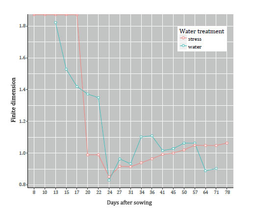
Figure 3. Finite dimension of roots (Leptochloa crinita), with different water treatments.

Figura 3. Dimensión finita de raíces (Leptochloa crinita), con distintas condiciones de riego.

The finite dimension of both roots decreases in 8 - 24. The first five values of the red line are at the top of the diagram which means, for the software used (the statistical software R), that the value is infinite. This says that the root is not ramified in this period. When it does ramify the finite dimension becomes finite and goes down. Not surprisingly, since both are of the same species, the blue one also decreases in this period and, indeed, reaches almost the same minimal value (around .84). We should also remark that these roots are far longer than wider, so that their diameters are achieved at soil-point to deepest endpoint.

Most interesting is the different behaviour of the roots in the period 24 - 78. While the red one (with little water) grows steadily, at almost constant pace, the blue one (with lots of water) goes up and down, almost periodically. The interpretation, using "What dim_f(Π) measures", is that the plant that received less water in this period (red line) prioritises lateral growth over growth in depth. The plant that received water at field capacity (blue line), on the other hand, keeps changing priorities: growth in depth over lateral growth, and then the opposite, and so on.

CONCLUSIONS AND FUTURE WORK

The results reported here show that dim f closely follows the ontogenesis of the aerial part and roots of the plants studied. Moreover, they clearly show the different growth strategies followed by plants. This is why we believe that dim_f(Π) is a good, objective measure of ontogenesis that, moreover, is reproducible because it is calculated with the same methodology for every type of foliage of plant or root. Our results suggest that each species has its own distinctive "signature".

This is a first, pioneering work in applying finite Hausdorff dimension to the study of plants. Our results are tentative because we have little empiric evidence. We have to study longer series of measurements, other species, other roots. This way we could prove or disprove our claims above, as well as elucidate, for instance, how dim _f(Π) reacts to different management practices, e.g. pruning. Silvicultural treatments applied to woody plants in arid zones still have a high degree of uncertainty (4, 16). We hypothesise that, after each practice, a plant tries to regain its "normal" finite dimension, as expressed in its finite dimensional "signature". These questions will surely lead us to a deeper understanding of how plants grow, and result in better management practices. In addition, if we can associate different functional traits with the finite dimension, it could become a tool to improve species in search of specific traits.

REFERENCES

1. Alonso, J. M. 2015. A Hausdorff dimension for finite sets. arXiv:1508.0294v1. 1-29.         [ Links ]

2. Alonso, J. M. 2016. A finite Hausdorff dimension for graphs. arXiv:1607.08130v1. 1-11.         [ Links ]

3. Alonso, J. M.; Arroyuelo, A.; Garay, P. G.; Martin, O. A.; Vila, J. A. 2018. Finite dimension: a mathematical tool to analise glycans. Scientific Reports. 8(1): 4426. DOI: 10.1038/ s41598-018-22575-4.         [ Links ]

4. Alvarez, J. A.; Villagra, P. E.; Villalba, R.; Debandi, G. 2013. Effects of the pruning intensity and tree size on multi-stemmed Prosopis flexuosa trees in the Central Monte, Argentina. Forest Ecology and Management. 310: 857-864.         [ Links ]

5. Berntson, G. M. 1994. Root systems and fractals: how reliable are calculations of fractal dimensions? Annals of Botany. 73: 281-284.         [ Links ]

6. Cavagnaro, J. B.; Lemes, J.; Ventura, J. L.; Passera, C. B. 1989. Variabilidad ecotípica y producción forrajera de Trichloris crinita. In: 14 Congreso de Producción Animal. Revista Asociación Argentina de Producción Animal.         [ Links ]

7. Falconer, K. 2003. 2nd ed. Fractal Geometry - Mathematical Foundations and Applications. John Wiley & Sons Ltd.         [ Links ]

8. Fitter, A. H.; Stickland, T. R. 1992. Fractal characterization of root system architecture. Functional Ecology. 6: 632-635.         [ Links ]

9. Gayon, J. 2000. History of the concept of allometry. American Zoologist. 40: 748-758.         [ Links ]

10. Glazier, D. S. 2005. Beyond the ’3/4-power law’: variation intra- and interspecific scaling of metabolic rate in animals. Biological Reviews. 80(4): 611-662.

11. Glazier, D. S. 2010. A unifying explanation for diverse metabolic scaling in animals and plants. Biological Reviews. 85(1): 111-138.         [ Links ]

12. Hallé, F.; Oldeman, R. A. A. 1970. 2nd ed. Essai sur l’architecture et dynamique de la croissance des arbres tropicaux. Mason and Co.

13. Hausdorff, F. 1919. Dimension und äußeres maß. Mathematische Annalen. 79: 157-179.         [ Links ]

14. Kleiber, M. 1932. Body size and metabolism. Hilgardia. 6: 315-351.         [ Links ]

15. Kleiber, M. 1947. Body size and metabolic rate. Physiological Reviews. 27: 511-541.         [ Links ]

16. Kozlowski, T. T.; Pallardy, S. G. 1997. 2nd ed. Physiology of Woody Plants. Academic Press. San Diego. California.         [ Links ]

17. Kozub, P. C.; Barboza, K.; Cavagnaro, J. B.; Cavagnaro, P. F. 2018. Development and characterization of SSR markers for Trichloris crinita using sequence data from related grass species. Revista de la Facultad de Ciencias Agrarias. Universidad Nacional de Cuyo. Mendoza. Argentina. 50(1): 1-16.         [ Links ]

18. Packard, G. C.; Birchard, G. F. 2008. Traditional allometric analysis fails to provide a valid predictive model for mammalian metabolic rates. The Journal of Experimental Biology, 211: 3581-3587.         [ Links ]

19. Petit, G.; Anfodillo, T. 2009. Plant physiology in theory and practice: An analysis of the web model for vascular plants. Journal of Theoretical Biology. 259(1): 1-4.         [ Links ]

20. Price, C. A.; Enquist, B. J.; Savage, V. M. 2007. A general model for allometric covariation in botanical form and function. Proceedings of the National Academy of Sciences of the United States of America. 104: 13204-13209.         [ Links ]

21. Price, C. A.; Weitz, J. S. 2012. Allometric covariation: a hallmark behavior of plants and leaves. New Phytologist. 193: 882-889.         [ Links ]

22. Reinhardt, D.; Kuhlemeier, C. 2002. Plant architecture. EMBO Reports. 3: 846-851. DOI: 10.1093/embo-reports/kvf177.         [ Links ]

23. Ruiz Leal, A. 1972. Aportes al inventario de los recursos naturales renovables de la Provincia de Mendoza - Flora Popular Mendocina. Deserta. 3: 1-299.         [ Links ]

24. Savage, V. M.; Gillooly, J. F.; West, G. B.; Allen, A. P.; Enquist, B. J.; Brown, J. H. 2004. The predominance of quarter-power scaling in biology. Functional Ecology, 18: 257-282.         [ Links ]

25. Savage, V. M.; Deeds, E. J.; Fontana, W. 2008. Sizing up allometric scaling theory. PLoS Computational Biology. 4: 1-17.         [ Links ]

26. Schopfer, P. 1995. Plant physiology. Springer Verlag. Berlin.         [ Links ]

27. Tatsumi, J.; Yamauchi, A.; Kono, Y. 1989. Fractal analysis of plant root systems. Annals of Botany. 64: 499-503.         [ Links ]

28. Wang, H.; Siopongco, J.; Wade, L. J.; Yamauchi, A. 2009. Fractal analysis on root systems of rice plants in response to drought stress. Environmental and Experimental Botany. 65: 338-344.         [ Links ]

29. West, G. B.; Brown, J. H.; Enquist, B. J. 1997. A general model for the origin of allometric scaling laws in biology. Science. 276: 122-126.         [ Links ]

30. West, G. B.; Brown, J. H.; Enquist, B. J. 1999a. A general model for the structure and allometry of plant vascular systems. Nature. 400: 664-667.         [ Links ]

31. West, G. B.; Brown, J. H.; Enquist, B. J. 1999b. The fourth dimension of life: Fractal geometry and allometric scaling in organisms. Science. 284: 1677-1679.         [ Links ]

ACKNOWLEDGEMENTS

We thank Hugo Debandi for his help and Julio Cristaldo for the meteorological records. We thank the referees for their helpful suggestions.

This work was completed with the support of a Research Scholarship of Universidad Nacional de Cuyo (SeCTyP).