Introduction

Forestry decision-making is often based mainly on stand growth and yield ¹⁴, and the prediction of these variables has been under constant study. At present, stand growth and yield are predicted with mathematical models in function of state variables such as number of trees, basal area, dominant height, and others ¹⁰. In growth models, the number of trees per unit of area is expressed in terms of mortality or survival ⁸. Stand mortality is a key component of growth and yield models, and its prediction is essential for obtaining precise estimates of state variables such as volume and biomass.

Modeling mortality can be done at the individual tree or surface unit levels. The first option is difficult due to its high variability ^8,20,21,26, and this problem is augmented by a limited database and when a wide range of growing conditions is not available ⁹. Modeling mortality at the stand level, however, is more robust since it only considers mortality generated by competition, excluding mortality generated by causes such as attacks by biological or other external agents ^7,8,12.

Modeling mortality at the individual tree level is generally done with logistics models ^{6,17,24,25,26}. At the surface unit level, probability equations of the shape P = (1+ e ^βX ) ^-1 are used, where βX is a linear combination of parameters b _i and state variables of stand x _i , including crop age, average square diameter (D _q ), crown diameter, average height, and dominant height. Another way to model mortality at the surface unit level is with difference equations. This alternative involves the relative mortality rate (∂N /∂E), which is assumed to be closely related to the current stand age ( E ), density in a previous period ( N ), and site quality ^3,5,27. Although relative mortality rates are generally related to various stand state variables such as stand density, age, dominant height, basal area, DQ, volume, and biomass, the literature recommends avoiding the use of variables derived from trunk diameter (basal area, Dq, volume, biomass) as interventions like thinning substantially weaken the relationship of these variables with stand density ^8,12.

In several studies, mortality has been modeled at the surface unit level using either difference equations or survival probability equations. Zhao et al. (2007) noted that both require taking measurements throughout crop life and that long periods of time may pass in which no mortality is recorded in the stand, leading to a lack of convergence for these models ²⁴. The properties of difference equations include consistency, mortality rates lacking variance, and near-zero asymptotic limits of stand density ^3,24,27. The research presented in this paper was carried out with traditional crops, i.e., in stands created for sawable or pulpable products and, to date, no such research has been published regarding crops for biomass production for dendroenergetic generation. Intraspecific competition mainly for water and nutrients should occur much earlier for short-rotation crops, usually established in high-density plantations, than for traditional crops. Therefore, the former should also manifest individual mortality at earlier ages.

In Chile, crops intended for biomass production have only been established recently in experimental areas. Crop potential for operational scale and the best strategy for growth and yield projection remain unknown. The objective of this paper is to model stand mortality in the first 40 months of growth for three dendroenergetic crops: Acacia melanoxylon R. Br., Eucalyptus camaldulensis Dehnh., and Eucalyptus nitens (Deane & Maiden), established at plantation densities of 5,000, 7,500, and 10,000 trees ha^-1.

Material and methods

Modeling mortality

We modeled mortality at two levels, first using individual tree and stand data. For indi vidual trees, we used the logistics model approach in the form of P = e ^βX / (1+ e ^βX ). In this equation, βX is a linear combination of individual tree variables at current time t and previous time t −1, βX= b ₁ΔIC + b₂ Δg + b₃ E+ b _N I _N . Here, ΔIC is the competition index variation between the current growth period and the previous one. Likewise, Δg is the variation of basal area growth in both periods, E is age expressed in months and I _N the stocks incorporated as dummy variable. The competition index was calculated using the Hegyi model ¹¹ and implemented via the Siplab package in R software ⁹. Δg was calcu lated according to differences between average increment and the last period’s increment in total height ((h _t - h _t-1 ) / (E _t - E _t-1 )) / (h _{t-1 /} E _t-1 ). We postulated the growth rate decrease and hence the competition index in measurement to instance t −1 would be an estimator of mortality in later instance t . The logistics model was set to classify the death of a tree with a probability value less than 0.5.

We followed two routes for mortality modeling at the stand level. One comprised survival probability models, i.e. P = (1+ e ^βX ) ^-1 , where P represents the proportion of live trees in each plot in relation to the 49 initially established ones, and βX is the linear combination of parameters βˆ and independent variables X to estimate X . For linear combinations of βX in the survival probability models, we used equations:

(1)

(2)

(3)

(4)

where:

E = the age of the crop expressed in months,

D _q = the mean square diameter,

H _dom = the dominant height,

b ₀, b ₁, b ₂, and b ₃ = the parameters to estimate. Dominant height was calculated as the average height of the five trees with the greatest D per plot.

Difference equations were also used to model mortality. Zhao et al. (2007) related relative mortality to age and/or site quality, following the (∂N /∂E)/ N= αN ^β f (site) f (age) shape, an equation in which ∂N /∂E represents the mortality rate at age E, f (site) and f (age) are functions of site quality and age, respectively, and α and β are param eters. We analyzed eight of the 28 models proposed by Zhao et al. (2007) for modeling mortality in the trial. Only one site was used in this study; thus, the expression was reduced to (∂N /∂E)/ N= αN ^β f (age). Moreover, assuming the relative mortality rate was not related to age ( f (age) =1) and that its decline was independent of plantation density (β = 0), the expression of mortality rate (∂N /∂E)/ N= αN ^β f (site) f (age) was reduced to(∂N /∂E)/ N= α, implying the relative mortality rate was constant (α ) at any age. In its initial condition, this expression was N = N ₁ when E = E1 and should be the difference equation for predicting N = N2 at E = E2. Therefore, inte grating d N / N = αdE , we got N = e ^(αE) and evaluating the difference equation we got N ₂ = N ₁ e ^{b1(E2 - E1)} (model [1]). In models [2] to [8], the initial assumption changed regarding the relative mortality rate, but its development was identical. All these functions were used previously to model mortality in adult stands with densities ranging from 740 to 1,970 trees ha^{-1 (4,15,16} (Table 1, page 147).

Table 1: Tabla 1: Mathematical expressions of difference equations and their respective mortality models. Expresiones matemáticas de las ecuaciones diferenciales y sus respectivos modelos de mortalidad. 

To determine the level of intraspecific competition to which the trial was subjected, we analyzed the relationship of stand density-D _q following the methodology proposed by Wittwer et al. (1997). These authors suggested incrementing the intercept 1.96 times the standard deviation of the model to determine the mortality curve of the maximum site load. The fitting were done for each species and plantation density.

Results

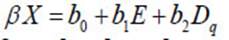
Individual tree modeling showed potential to predict the mortality rate, with the ΔIC and Δg variables being significant, denoting that those variables were valid estimators in the model, also permitting describing the dynamic of the competition index in successive periods (Figure 1).

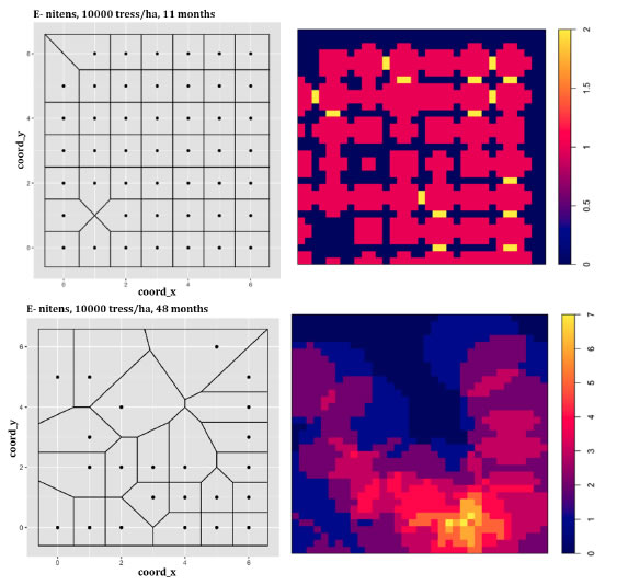
Figure 1: Figura 1: Left: Voronoi triangulation for E. nitens; the available space to grow at initial density of 10,000 trees ha^-1 for ages of 11 and 48 months. Right: Heatmap for the Hegyi competition index in both growth periods. Izquierda: Triangulación de Voronoi para E. nitens; espacio disponible para crecer en la densidad de plantación de 10.000 árboles ha^-1 para la edad de 11 y 48 meses. Derecha: Mapa de calor para el índice de competencia de Hegyi en ambos periodos de crecimiento. 

This approach allowed to fit a model by species, and the different planta tions were incorporated as dummy variables. The best modeling accuracy was achieved for A. melanoxylon with 88.6%, followed by E. camaldulensis and E. nitens (Table 2, page 149).

Table 2: Tabla 2: Estimated parameters for the individual tree mortality model. Parámetros estimados para el modelo de mortalidad de árboles individuales. 

For all species, the model showed better performance to estimate living trees than dead trees, expressed as positive prediction value (PPV), as opposed to negative prediction value (NPV). In the case for E. camaldulensis, the model’s performance to estimate individual tree mortality was deficient, achieving only 23.7% of accuracy. Although the individual tree method had high accuracy and good ability to estimate live tress, NPV values suggested discarding this analysis approach.

Although model [4] was the most precise of the probability equations (Table 3, page 150), followed consecutively by models [2], [1], and [3], model [2] was the most appropriate for modeling survival probability in terms of parsimony, followed by models [1], [4], and [3].

Table 3: Tabla 3: Estimated parameters using the method of estimating survival probability equations. Parámetros estimados utilizando el método de estimación de ecuaciones de probabilidad de supervivencia. 

Although model [4] was more precise, it required the estimation of four parameters, which is one more than model [2], indicating that Hdom was not a variable that, in the presence of the age and D _q variables, significantly reduced the estimation error. Mortality modeling using this methodology presented many non-significant estimates of the param eters. Apparently, the applicability of this method was conditioned by the number of obser vations. In this study, variables were only measured eight times, the last time 40 months after establishing the trial. These scant measurements caused the limited significance of the parameters estimated in the mortality probability equations.

Age was the variable with the greatest explanatory capacity in the survival probability equations (Table 3, page 150). Although model [1] did not have the best precision indicators (RMSE), its results were similar to those obtained by model [2] in terms of parsimony (AIC), with age and D _q incorporated into its polynomial. In model [1], parameter b ₁, associated with crop age, was significant in most cases. When incorporating other predictive variables into the survival probability models ([2], [3], [4]), no parameter was significant.

Model [1], with which we obtained the best results in terms of parsimony, showed that the probability of survival varied between plantation densities and had an inverse relationship with plantation density (Table 3, page 150). The results only indicated a significant effect of density on the model parameters for the Eucalyptus species, and an independent fitting was required for each level of plantation density. Nonetheless, for E. camaldulensis, the lack of convergence of the model affected the interpretation of the test and the suggestion of fitting for each plantation density of this species should not be considered, since the observed mortality rate was low and null for 5,000 trees ha^-1 (Table 3, page 150 y Figure 2, page 151).

Figure 2: Figura 2: Mortality modeling based on the survival probability functions for models 1 (O), 2 (▲), and 4 (■) and the difference equations for models 5 (O), 6 (▲), and 7 (■). Modelación de la mortalidad basada en las funciones de probabilidad de supervivencia para los modelos 1 (O), 2 (▲) y 4 (■) y ecuaciones diferenciales para los modelos 5 (O), 6 (▲) y 7 (■). 

Difference equation [5] showed the best results for both precision and parsimony (Table 4, page 152), followed by models [7] and [6], which gave good RMSE and AIC indicators.

Table 4: Tabla 4: Estimated parameters in the best three fitted models using the difference equations method. Parámetros estimados en los tres mejores modelos ajustados mediante el método de ecuaciones diferenciales 

Table 4 (page 152) shows only the three best fits obtained; the results of models [8] and [9] were excluded due to low precision, as were the results of models [10], [11], and [12], which had convergence problems, likely due to the high number of parameters in the models and the scant number of measurements available. Despite these limitations, difference equation [5] modeled satisfactorily the decline in tree numbers, and all its parameters were signif icant. In general, the models of the difference equations that converged showed mostly significant parameters.

Observed relative mortality rate remained constant during the first 40 months of growth, i.e., (∂N /∂E) / N= α. This assumption was implicit in model [5] (Table 4, page 152) and, therefore, this equation sufficed for obtaining precise mortality rate estimates. Model [7], which showed precision and parsimony indicators similar to model [5], assumed a relative mortality rate of (∂N /∂E) / N= α + β / E. This assumption was adequate for predicting the mortality rate, although the estimation of this model showed a greater error. Model [6] was also fitted satisfactorily but showed greater prediction errors, assuming the relative mortality rate varied non-linearly in the function of crop age ((∂N /∂E )/ N= αE ^β). Therefore, of the eight difference equations tested, model [5] yielded the most precise for the first 40 months of growth, indicating that mortality was constant regardless of age. The precision of functions [6] and [7] was probably obscured by the scant number of observations available. Logically, mortality should be closely related to crop age, whether expressed in shape change or slope change that would eventually be manifested at some age of the crop. This effect was implicit in these equations.

In general, precision (RMSE and AIC) diminished along with plantation density, a result shown in the three best difference equations (Table 4, page 152). Of these, model [5] indi cated an inverse relationship of parameter b ₁ with plantation density. This was shown by the greater relative mortality rate at the highest plantation densities, which was reasonable if we assumed greater intraspecific competition, which conditions crop survival, on plots established with more trees per surface unit. The effect of plantation density on the param eters of model [5] was manifested in this tendency, but no significant reduction of the residual variation in the fitted models independently by plantation density levels was found in relation to average fitting. Therefore, up to 40 months of age, modeling mortality through difference equations could be done by averaging, i.e., without considering the effect of the plantation density.

Some equations were deficient at estimating mortality in the first growth stages (Figure 2). Model [4] underestimated the number of A. melanoxylon trees at the time of establishing the crop. For this same species, model [1], the most precise of the probability equations, overestimated density in the first growth stages at densities of 7,500 and 10,000 trees ha^-1. In those cases, restricting the estimate to the value of the nominal stand density caused the curve to flatten. On the contrary, the difference equations did not underestimate the tree numbers at the time of establishing the plantation for any of the three species, although this type of model did register cases of overestimation in the first growth stages, for example for A. melanoxylon and E. nitens. Normally, mortality was not generated in the crops’ early stages due to a lack of competition. However, semi-annual records of these rapidly growing crops revealed a strong rather than a gradual decline in the number of trees between the fourth and fifth measurements, i.e., 16 to 23 months after establishment (Figure 2). This hindered the predictive capacity of both the probability and the difference equation models, leading to underestimating tree numbers when there was no mortality.

Discussion

The best method for modeling mortality in these dendroenergetic trials was with models derived from difference equations. These models, in general, presented greater precision of fit and showed a greater number of significant parameters. The mortality models derived from the probability functions presented many non-significant parameters. Therefore, the estimates were not reliable and had limited applicability in growth and yield models. The difference equations also presented non-significant parameters, but a lesser number. This inconvenience was apparently connected to the number of observations available for the study, since the hypothesis tests for the parameters in the non-linear models were known to be strongly conditioned by sample size ¹⁹.

Other authors have also evaluated the two alternatives for modeling the mortality analyzed here. For example, Zhao et al. (2007) modeled the probability of survival based on a proba bility model using age, basal area, site index, and stand density from the immediately preceding measurement period as predictive variables; all the parameters were found to be significant. Based on those results, the authors recommended only incorporating age and basal area as predictive variables in survival probability models, since this latter variable indicated the competition level. The results of that study were in agreement with ours, since our best model contained the explanatory variables age and D _q as a competition indicator. The recommendation of other authors to avoid the use of expressions derived from the diameter (e.g. D _q or basal area), since these variables are highly susceptible to forestry interventions ⁸, did not apply to this type of crop as it was not subjected to forestry interventions such as thinning. Nor did the use of dominant height seem advisable when dealing with crops destined for biomass production. The utility of this variable is dubious, considering that the proportion of trees is not a clear indicator of site quality due to crop age. At early ages, the intrinsic quality of the site did not show in tree growth. Rather, activities such as site preparation and/or other forestry activities were the main factors that condition early-age crop establishment, growth, and survival.

Although this study obtained similar precision with both methods, the best difference equation [5] was more precise than the best survival probability equation [2]. Therefore, we recommend using models based on difference equations to model the mortality of crops intended for dendroenergetic generation. Moreover, study results showed these models had an advantage over the survival probability models in terms of parsimony and the number of significant parameters. Zhao et al. (2007) evaluated these two alternatives in adult stands of Pinus taeda Engelm., establishing good precision results with difference equa tions. In this study, the best results were obtained using the ((∂N /∂E )/ N= (c ₀ + c ₁)N ^βδ ^E ) and ((∂N /∂E )/ N= N ^β / αSite + δ / E models. Given that the current study was conducted at only one site, it was not possible to incorporate site quality as a predictive variable in the difference equation. Therefore, the best results were obtained assuming the relative mortality rate was proportional to age in the shapes of (∂N /∂E )/ N= α =∂∂N EN / / and (∂N /∂E )/ N= αE ^β . These assump tions also were in line with other studies, in which, given the objective of simplifying the development of mortality models, it was assumed that relative mortality rates were inde pendent of site quality ^1,13.

No mortality was recorded in the first measurement carried out in this study, like what happened with adult stands: often, during long intervals of time in the first growth stages, no crop mortality was registered. Between 36.7% and 44.6% of initial time intervals did not show mortality, according to Zhao et al. (2007). The authors noted that this problem was the main cause of a lack of convergence in the non-linear mortality models. Woollons (1998) recommended extracting data that do not present mortality, since these complicate the estimation and can cause the model to underestimate the stand’s mortality rate. Other authors noted that by maintaining only the information presented by mortality, the model can overestimate the mortality rate ^6,24. In this study, the longitudinal extraction of infor mation was not required since mortality was manifested as of the fourth month of the trial.

Mortality rates observed for this crop varied widely between species (Figure 3, page 154).

Figure 3: Figura 3: Relationship between average and maximum size-density (solid line = stand density index maximum; dashed line = stand density index average). Relación entre tamaño-densidad media y máxima (línea sólida = índice de densidad del rodal máximo; línea segmentada = índice promedio de densidad del rodal. 

The experimental units established with E. camaldulensis showed the lowest mortality rates, followed by A. melanoxylon and E. nitens. Apparently, E. nitens showed the highest level of stress due to strong intraspecific competition, which was expressed in greater mortality rates. The model proposed by Wittwer et al. (1997) indicated that the slope of the relationship of density-D _q in A. melanoxylon was -0.015, -0.062, and -0.204 for 5,000, 7,500, and 10,000 trees ha^-1, respectively, and -0.286, -0.311, and -0.393 for 5,000, 7,500, and 10,000 trees ha-1 for E. nitens, respectively. For E. camaldulensis, slope value was close to zero, since mortality for this species was near zero (Figure 3, page 154). But these results were heavily conditioned by the high persistence of these species. Empirical data from this trial showed a large proportion of individuals in a clearly suppressed social class. Sandoval et al. (2012) analyzed the evolution of the diameter distributions in this trial, reporting that the distribution tended to be more platykurtic in the measure that the crop grew, but small er-diameter classes were constantly causing a skew towards the left of the distribution. This revealed the high persistence of these species, which conditioned the relationship of stand density with size and allowed the observed mortality to be attributed to the levels of intra specific competition generated in the trial.

Conclusions

Forty months after the establishment of the crop, E. camaldulensis was the species that had the greatest survival rate, followed by A. melanoxylon and E. nitens. Evidently, E. camal dulensis is a highly persistent species, unlike the other two. Nonetheless, another study conducted with these crops showed low biomass yields for E. camaldulensis and A. mela noxylon, indicating that, despite the high mortality rates of E. nitens, this is an interesting species to consider for establishment as a dendroenergetic crop.

The mortality models derived from difference equations showed, in general, greater precision than the survival probability equations. The former was also advantageous in terms of parameter significance. Therefore, study results indicated that difference equa tions should be used for modeling the mortality of crops intended for dendroenergetic purposes. The survival probability equations showed estimation difficulties, apparently due to the limited number of observations.

Of the eight difference equations tested, model [5] was the most appropriate for modeling the mortality of dendroenergetic crops. Although models [5], [6], and [7] presented a similar estimation error, model [5] surpassed them in terms of parsimony. These results showed that the relative mortality rate remained constant, which was well-described by relationship (∂N / ∂E) / N = α.

There was no statistical evidence of a significant effect of plantation density on the mortality models based on the difference equations. Plantation density level fitting was not justified in the three best models. The results showed a constant relative mortality rate, which indicated that the rate of decline in number of trees was similar between plantation densities. Although the results clearly showed that the rate of decline in the number of trees increased at greater plantation density, this difference was slight and not significant. Moreover, this result was probably also influenced by the high variability of the information registered at this stage of the crop.

The relative mortality rate was well modeled by difference equation [5], which assumed a constant, predictable decline in the number of trees based on crop age. Density-size rela tionship analysis showed the site was still not at its maximum load capacity. Nonetheless, this result was heavily conditioned by the high level of persistence of the species. Therefore, mortality modeling is recommended for crops established at high plantation densities and, with these species, this may be done following a classification of the social stratum, excluding suppressed trees from the analysis. Thus, including dead and suppressed trees as “social mortality” could improve the density-size relationship and the estimate of the number of live trees would then concentrate on individuals of greater interest in terms of biomass yield.