


Servicios Personalizados
Revista

Articulo
 Inglés (pdf)
 Articulo en XML
 Referencias del artículo
 Enviar articulo por email
Indicadores
-
 Citado por SciELO
Links relacionados
-
 Similares en
SciELO
Similares en
SciELO
Compartir

 Permalink
Latin American applied research
versión impresa ISSN 0327-0793
Lat. Am. appl. res. vol.41 no.3 Bahía Blanca jul. 2011
Behavior of the solution of the two-phase stefan problem with regard to the changing of themal coefficients of the substance
M. C. Olguin†, M. C. Sanziel‡ and D. A. Tarzia*
† Dto. de Matemática, Fac. de Cs. Exactas, Ing. y Agrimensura, Univ. Nac. de Rosario,
(S2000BTP) Rosario, Argentina. mcolguin@fceia.unr.edu.ar
‡ Consejo de Investigaciones, Dto. de Matemática, Fac. de Cs. Exactas, Ing. y Agrimensura,
Univ. Nac. de Rosario, (S2000BTP) Rosario, Argentina. sanziel@fceia.unr.edu.ar
* Dto. de Matemática FCE, Univ. Austral-CONICET, (S2000FZF) Rosario, Argentina
DTarzia@austral.edu.ar
Abstract - We consider one-dimensional two-phase Stefan problems for a finite substance with different boundary conditions at the fxed faces. The goal of this paper is to determine the behavior of the free boundary and the temperature when the thermal coefcients of the material change.
We obtain properties of monotony with respect to the latent heat, the common mass density, the specifc heat of each phase and the thermal conductivity of the liquid phase.
We show that the solution is not monotone with respect to the thermal conductivity of solid phase, in some cases, by computing a numerical solution through a finite difference scheme.
The results obtained are important in technological applications as the climate of buildings, the storage of energy in satellites and clothes and the transport of biological substances and telecommunications.
Keywords - Phase change material; Two phase Stefan problem; Finite difference method
I. INTRODUCTION
Several technological applications can be modeled through heat transfer problems with phase-change. The Phase Change Materials (PCMs) are substances whose phase-change temperature make them available to moderate oscillations of temperature and to store energy of another substance in contact with them (Jiji and Gaye, 2006). For this reason PCMs are used for the climate of buildings, the storage of energy in satellites and clothes and the transport of biological substances (Asako et al., 2002; Lamberg and Sirn, 2003), among a variety of applications.
Usually, the technological way to select a PCM is through its phase-change temperature, but when there are several products in the correct range of temperature, it is necessary to study another properties of the substance, for example the thermal coefcients, in order to choose the most convenient PCM.
When we consider a packaging of a PCM that recovers an organic substance to be transported, it is essential to find the thickness of this pack to insure the optimal temperature of conservation in the organic substance during total time of transport (Bouciguez et al., 2001; Farid et al., 2004; Medina et al., 2004; Zalba et al., 2003; Zivkovic and Fujii, 2001). Because the sizes of the pack (wide, length and height) are sufciently greater than its thickness, we can assume that the heat transfer occurs in only one direction. Moreover, if we consider a material with one portion at solid state and the other at the liquid state, and take into account the environment conditions, we have an one dimensional two-phase Stefan problem (Lamberg, 2004; Lamberg et al., 2004).
In Olgu´ın et al. (2007), we considered a onedimensional one-phase Stefan problem for fusion of a semi-infinite material. We showed that, both, the temperature and the free boundary present a monotonous behavior with respect to the latent heat, the mass density and the specifc heat. We also showed that the solution is not monotone with respect to the thermal conductivity.
At the present work we continue this line of research. We consider several two-phase one-dimensional Stefan problems for a finite material, with different boundary conditions at the two fxed faces, in order to determine the behavior of the solutions when the thermal coefcients change.
In Section 2 we study a phase-change problem with temperature specifcation on both fxed faces of the finite material and we obtain results of monotony for latent heat, mass density, specifc heat of the solid and the liquid phase, and thermal conductivity of the liquid phase, by using the maximum principle (Protter and Weinberger, 1967).
Analogous results are obtained in Section 3, by considering heat flux specifcation at both fixed faces of the finite material and, in Section 4, with temperature specification at the left fixed face and a heat flux specifcation at the right fxed face.
When we consider the thermal conductivity of the solid phase, it was not possible to establish analytical results of monotony. In order to obtain some conclusion for this case, in Section 5 we consider a numerical solution. Since the free boundary change with time, the domain of the problems is variable, then it is necessary to develop a particular scheme with a time variable mesh. We can show that, in some cases, the solutions are not monotone.
II. PROBLEM WITH TEMPERATURE
BOUNDARY SPECIFICATION AT BOTH FACES
A. Mathematical problem and preliminary results
We consider a finite material represented by the interval [0, 1]. At the initial time, we suppose that one portion of the material is at solid phase and the other is at liquid phase. If we consider that s(t) is the position of the free boundary at each time and

is the temperature of the material, the problem (P1) is to find functions w(x, t), s(t) and a time T > 0, so that they satisfy the following conditions:
 | (1) |
 | (2) |
 | (3) |
 | (4) |
 | (5) |
 | (6) |
 | (7) |
 | (8) |
 | (9) |
where  is the thermal diffusivity of the phase i (i = s, l) and φ(b) = 0 =
  (b) (see Fig.1).

Figure 1: Scheme of the problem (P1)
In Cannon and Primicerio (1971), Tarzia (1987) and Cannon (1984), under suitable hypothesis for data, it was proved that:
*) there is a unique solution for problem (P 1) for all T > 0;
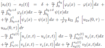
**) the Stefan condition (Eq.6) is equivalent to the integral equation:
 | |
 | (10) |
where
B. Analytical results of monotony
In this Section we use the maximum principle, Hopf's lemma (Protter and Weinberger, 1967; Cannon, 1984) and the result of the following Lemma, when it is required, in order to establish some properties of monotony for the solution of problem (P 1).
Lemma 1 Let w be the solution of (P 1). Then:
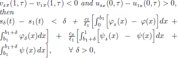
i) ux(s(t),t) < 0 and vx(s(t),t) < 0 for t > 0;
ii) If the function f (t) is continuously differentiable for t > 0 and φ(x) is twice continuously differentiable at  and
and  then
then for 0 < x < s(t), 0 < t < T .
iii) If g(t) is continuously differentiable for t > 0 and  is twice continuously differentiable at
  and
and  then
then  for s(t) < x < 1, 0 < t < T .
Proof.
i) The results are obtained when the maximum principle and Hopf ' s lemma are applied to functions u and v respectively.
ii) We define the auxiliary function z = uxx which verify the associated problem

By using the maximum principle, we obtain z ≥ 0.
iii) The proof follows (ii) by defining now the auxiliary function z = vxx.
Proposition 2 The solution {w(x, t), s(t)} of problem (P 1) depends monotonically on the latent heat  , the mass density ρ, the specific heat ci (i = s, l) and the thermal conductivity of the liquid phase kl.
Proof. The five results are similar but the proofs are different because we must change the coefficients only in the Stefan condition for the latent heat , only in the heat equation for the specific heats ci(i = s, l) and in both equations in the remaining cases.
a) We consider  . We call {w1, s1}, {w2, s2}the solutions of problem (P 1) with
  and si (0) = bi for i =1, 2. We consider two cases: s1(0) >s2(0) and s1(0) ≥ s2(0).
Case I: Let b1 = s1(0) >s2(0) = b2. We suppose t0 is the first time such that s1(t0)= s2(t0) and s2(t) < s1(t) for all 0 < t < t0. Because of that, it must occur (Fig.2):
 | (11) |

Figure 2: Free boundaries for
If we define the functions

for 0 ≤ t ≤ t0, then U satisfies the following conditions:
 | (12) |
 | (13) |
 | (14) |
 | (15) |
 | (16) |
By the minimum principle, condition (Eq.15) holds and then U ≥ 0 in 0 ≤ x ≤ s2(t), 0 ≤ t ≤ t0. At the point x = s1(t0)= s2(t0),we have U (s2(t0), t0) = 0, therefore U attains a minimum at (s2(t0), t0). By the Hopf's lemma, we have
 | (17) |
On the other hand, the function V , satisfies the following conditions:
 | (18) |
 | (19) |
 | (20) |
 | (21) |
 | (22) |
In a similar way as above, we obtain that V (x, t) ≥ 0 in s1(t) ≤ x ≤ 1, 0 ≤ t ≤ t0. Taking into account that V (s1(t0),t0)=0, then V has a minimum at (s1(t0),t0) and from the Hopf ' s lemma, it results
 | (23) |
But, from the Stefan condition (Eq.6), (Eq.11) and (Eq.17) we obtain:

which is a contradiction with (Eq.23). Then we conclude that:

for 0 ≤ t ≤ T .
Case II: We consider now b1 = s1(0) ≥ s2(0) = b2. Let δ > 0, then b2 ≤ b1 < b1 + δ. Let wδ ,sδ be the solution of (P1) whit latent heat  1 and sδ(0) = b1 + δ in (Eq.9). We define the functions
  and
and  on the intervals[0, b1 + δ] and [b1 + δ, 1]respectively by:
and

From case I, we have that:

Taking into account the Stefan condition (Eq.10) for s1 and sδ, and from Case I, it results that:

If we apply again the maximum principle and Hopf's lemma, we can see that:
which implies

Taking the limit when δ → 0, we have that s2 ≤ s1 in the common domain of existence. To complete the proof, we consider for i =1, 2
As we have seen before, w1 − w2 ≥ 0 for 0 ≤ x ≤ s2(t) and s1(t) ≤ x ≤ 1. For s2(t) ≤ x ≤ s1(t), we have w1(x, t) − w2(x, t)= u1(x, t) − v2(x, t) ≥ 0, because u1 ≥ 0 and v2 ≤ 0 and the thesis holds.
b) Now, we consider that the thermal conductivity of the liquid phase changes. Let kl1 < kl2 and we note as {w1, s1}, {w2, s2} the solutions of problem (P 1) with  and si(0) = bi for i =1, 2. As before, we consider two cases: s1(0) > s2(0) and s1(0) ≥ s2(0).
Case I: b1 = s1(0) < s2(0) = b2 and t0 is the first time such that s1(t0)= s2(t0), then we have (see Fig.3):
 | (24) |

Figure 3: Free boundaries for kl1 < kl2
If we define the function

we see that U satisfies the following conditions:
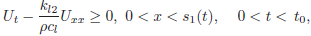 | (25) |
 | (26) |
 | (27) |
 | (28) |
 | (29) |
The inequality (Eq.25) is a consequence of part (ii) of Lemma 1, while the condition (Eq.28) is obtained from the minimum principle and then we conclude that U ≥ 0 in 0 ≤ x ≤ s1(t), 0 ≤ t ≤ t0. At x = s1(t0)= s2(t0), we have U(s1(t0), t0)=0, then U has a minimum at (s1(t0), t0) and from the Hopf's lemma, it results
 | (30) |
On the other hand, the function V satisfies the following conditions:
 | (31) |
 | (32) |
 | (33) |
 | (34) |
 | (35) |
In the same way as above, we have that V (x, t) ≥ 0 in s2(t) ≤ x ≤ 1, 0 ≤ t ≤ t0. Since V (s2(t0),t0)= 0, V has a minimum at (s2(t0),t0)and from Hopf's lemma, it results
 | (36) |
Therefore, from the Stefan condition (Eq.6), (Eq.24), (Eq.30) and Lemma 1 (i) we have:

which is a contradiction with (Eq.36). Then we conclude that:

for 0≤ t≤ T.
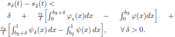
Case II: Let b1 = s1(0) ≤ s2(0) = b2. Let δ > 0, then b1 ≤ b2 < b2 + δ. We note {wδ,sδ} the solution of the problem (P1) with thermal conductivity of liquid phase kl2and sδ(0) = b2 + δ. We define the functions φδand  on the intervals [0, b2 + δ] and [b2 + δ, 1] respectively by:

From case I, we have that:
From the Stefan integral condition (Eq.10) for s2 and sδ and Case I we obtain:

If we apply the maximum principle and Hopf 's lemma, we obtain that
 | and |
 |
and consequently:
When δ tends to zero, we obtain that s1(t) ≤ s2(t) in the common domain of existence.
c) By a similar argument as above, applying the maximum principle and the Hopf 's lemma when it is necessary, we obtain the thesis taking into account that in this case the specific heat of each phase changes. We must consider that in this situation the heat equations (Eq.1) or (Eq.2) are affected.
d) As in c), when the mass density changes, we can show the monotony considering that the heat equations (Eq.1), (Eq.2) and also the Stefan condition (Eq.6) are affected.
III. PROBLEM WITH FLUX BOUNDARY SPECIFICATION AT BOTH FACES
A. Mathematical problem and preliminary results
We consider a similar problem to (P1), but on x = 0 and on x = 1 the conditions (Eq.3) and (Eq.4) are replaced by heat flux conditions respectively. Then, we define the problem (P2) for equations (Eq.1), (Eq.2), (Eq.5) − (Eq.9) and
 | (37) |
 | (38) |
In Tarzia (1987), Cannon (1971) and Cannon (1984) under certain hypotheses, it was proved that: *) there is unique solution for problem (P2) in 0 < t < T0, for some T0 > 0;
**) the condition (Eq.6) is equivalent to the integral equation for all t ≥ 0:
 | |
 | (39) |
where 
B. Analytical results of monotony
Proposition 3 Let {w(x, t), s(t)} be the solution of (P2). It depends monotonically on the latent heat , the mass density ρ, the specific heat ci (i = s, l) and the thermal conductivity of the liquid phase kl.
Proof.
a) When the latent heat changes, we consider two cases, as in the proof of Proposition 2:
Case I: b1 = s1(0) > s2(0) = b2 and
Case II:b1 = s1(0) ≥ s2(0) = b2.
In both cases we repeat the proof but we consider, for the auxiliary functions U and V , the following flux data:
Ux(0,t)=0, 0 < t < t0,
Vx(1,t)=0, 0 < t < t0.
In addition, in Case II, as before, we consider the functions φδ and on the intervals [0, b1 + δ] and [b1 + δ, 1] respectively by:

From the integral Stefan condition (Eq.39) for s1 and sδ and considering Case I we have:

and consequently:

Taking the limit as δ tends to 0, we obtain that s2 ≤ s1 in the common domain of existence. In order to complete the proof, we continue as in a) of Proposition 2.
The proof of the Proposition 3 for the other parameters is analogous to the cases b), c) and d) of Proposition 2.
IV. PROBLEM WITH TEMPERATURE SPECIFICATION ON x =0 AND FLUX SPECIFICATION ON x =1
A. Mathematical problem and preliminary results
We consider a similar problem to (P1), but on x = 0 and x = 1 the conditions Eq.(3) and Eq.(4) are replaced by temperature specification and heat flux condition respectively. Then, we define the problem (P3) for e Eqs.(1), (2), (5 − 9) and
| u(0,t)= f(t) > 0, 0 < t < T, | (40) |
| ksvx(1,t)= g(t) ≤ 0, 0 < t < T. | (41) |
In this case, under suitable hypothesis, it can be prove that the Stefan condition (Eq.6) is equivalent to the following integral equation for all t ≥ 0:
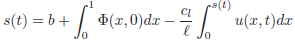 | (42) |
 |
where 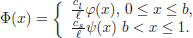
B. Analytical results of monotony
Proposition 4 Let {w(x, t),s(t)} be the solution of (P3). It depends monotonically on the latent heat, the mass density ρ, the specific heat ci(i = s, l) and the thermal conductivity of the liquid phase kl.
Proof.
a) We consider that the thermal conductivity of the liquid phase changes and, as in the proof of item b) of Proposition 2(b), we take into account two cases:
Case I: b1 = s1(0) <s2(0) = b2 and
Case II: b1 = s1(0) ≤ s2(0) = b2. We consider, for the auxiliary function V , a flux specification:
Vx(1,t)=0, 0 < t< t0,
and in Case II, as before, we consider the functions φδ and on the intervals[0, b2 + δ] and [b2 + δ, 1] respectively by:
 | and |
 |
From integral expression of the Stefan condition (Eq.42) for s2 and sδ and Case I we have:
By the maximum principle and the Hopf' s lemma, we obtain

which implies that

and consequently, if δ → 0, we obtain s1(t) ≤ s2(t) in the common domain of existence.
The proof for the other parameters is analogous to the Proposition 2.
Remark: We can not obtain any conclusion, through the maximum principle, about variations in the thermal conductivity ks of the solid phase. This case will be studied by a numerical approximation in Section 5.
V. NUMERICAL SOLUTIONS AND MONOTONY
A. Numerical scheme
In this section we propose a numerical method in order to approximate the solution {w(x, t),s(t)} of the problems P (q), for q =1, 2, 3. Since the free boundary change with time, the domain of the problem is variable. The numerical solution of free boundary problems of this type can be computed through different methods: front-traking methods and front-fixing methods (Zerroukat and Chatwin, 1994; Meyer, 1971; Crank, 1984). In this paper, we develop a scheme with a time variable mesh We propose a variable grid with fixed time step and with a constant number of space steps. These space steps will be update at each time level so that the free boundary is located on a node of the mesh (Fig. 4).
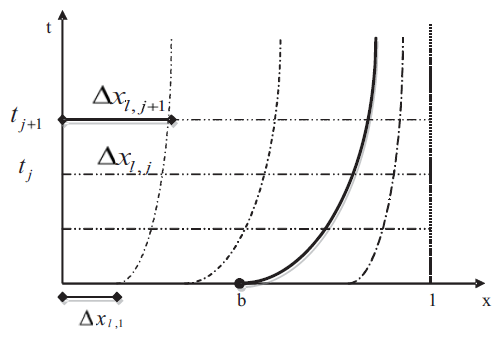
Figure 4: scheme for the time variable grid
We consider a fixed time step Δt and:
*) tj+1 = jΔt for j =0, 1, .., N.(N number of time intervals so that tN+1 ≤ T , time of coexistence of both phases).
*) For each time tj+1, we define a partition of [0, 1], and we take m steps in each phase as follow:
-in the liquid phase:
 ,
,
-in the solid phase:
 , in consequence

where  .
.
*)
*)
We define the coeficients:

where, we note  , and in each phase we approach the heat equation by an explicit finite difference scheme.
In order to approximate the distribution of temperature in (0, 1) x (0, T ) we replace equations (Eq.1) and (Eq.2) with j = 0, .., N by:
 | |
 | (43) |
| |
 | (44) |
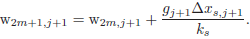
In an analogous way, we make the approximations of the boundary conditions:
for (P1): 
 | (45) |
for (P2): 
 | (46) |
for (P3): 
 | (47) |
We obtain the numerical solution through the following algorithm:
Step 1:
* Set the initial conditions and the boundary conditions
* Choose Δt > 0 and m;
Step 2: Set j =1
-compute  ,
,
-evaluate s'j from the Stefan condition (Eq.6),
-  (temperature on the free boundary),
-compute  , from (Eq.43) and (Eq.44),
-compute  from (Eq.45), (Eq.46) or (Eq.47) depending on the problem,
Step 3: While j ≤ N return to Step 2 with j = j + 1;
Remark: Since we use an explicit scheme, we must regard that the following four conditions are satisfied at each step, in order to have a convergent method:
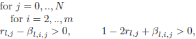
 The numerical solutions obtained from the above algorithm, are used to find counterexamples that show the nonmonotonicity of the solution with respect to the solid thermal conductivity. For this reason, any analysis about stability or convergence are done.
B. Numerical results
In order to analyze the monotony, we consider the numerical solutions of problem (Pq)(q =2, 3), for the thermal coefficients of water (Alexiades and Solomon, 1996):
* mass density ρ = 
* latent heat 
* thermal conductivity of liquid phase 
* thermal conductivity of solid phase 
* specific heat of the liquid phase 
* specific heat of the solid phase 
i) Problem (P2)
We consider the numerical solutions of problem (P2) for two different values of the thermal conductivity of the solid phase:  . For the initial conditions and the boundary conditions we take:

f(t)= −10; g(t)= −8;
and we choose Δt = 240seg and m = 25.
In Figure 5, we obtain a comparative graphic of the free boundary positions and in Figure 6 we show the temperature distribution at a fixed time t = 600hs.

Figure 5: Free boundary position (t ≤ 600h)

Figure 6: Temperature distribution at t = 600h
We can observe that the free boundary position have a monotone behavior but it does not occur for the temperature distributions.
For the numerical solutions of the problem (P 3) we consider the same values of the thermal conductivity of the solid phase as above. For the initial conditions and the boundary conditions we take:
 |  |
ii) Problem (P3)
 |  |
and we choose Δt = 240seg. and m = 25.
In Fig. 7, we obtain a comparative graphic of the free boundary positions, in Figure 8 we show the temperature distribution at a fixed time t = 276hs and in Figure 9 we zoom in Figure 8. We can observe that the free boundary position have a monotone behavior but it does not occur for the temperature distributions.

Figure 7: Free boundary position (t ≤ 276h)

Figure 8: Temperature distribution at t= 276 h

Figure 9: Temperature distribution at t= 276 h
VI. CONCLUSIONS
It was showed, through the maximum principle, that the solutions of two-phase one-dimensional Stefan problems for finite domains, depend monotonically on the latent heat, the mass density, the specific heat of each phase and the thermal conductivity of liquid phase when we consider the following boundary conditions:
1) temperature specification on both fixed faces;
2) flux specification on both fixed faces;
3) temperature specification on the left face and flux specification on the right face.
We developed a numerical scheme using finite difference methods with variable space step in order to obtain an approximate solution for those problems. We have showed, through those approximate solutions, that there is no monotony of the solution when the thermal conductivity of the solid phase changes for the problems with boundary conditions 2) and 3).
The monotony of the solution for the problem with temperature boundary condition on both fxed faces when the thermal conductivity of the solid phase changes, is at the moment, an open problem.
REFERENCES
1. Alexiades, V. and A.D. Solomon, Mathematical modeling of melting and freezing processes, Hemisphere-Taylor & Francis, Washington (1996). [ Links ]
2. Asako, Y., E. Gonçalves, M. Faghri and M. Charmchi, "Numerical solution of melting processes for fixed and unfixed phase change material in the presence of magnetic field-simulation of low-gravity environment ," Num. Heat Transf. Part A, 42, 565-583 (2002). [ Links ]
3. Bouciguez, A.C., L.T.Villa and M.A. Lara, "Análisis de sustancias de cambio de fase para su utilización en el envasado y transporte de productos alimenticios," VI Congreso Iberoamericano de aire acondicionado y refrigeración (2001). [ Links ]
4. Cannon, J.R. and M. Primicerio,"A two-phase Stefan problem with temperature boundary conditions," Annali Mat. Pura Appl., 88, 177-191 (1971). [ Links ]
5. Cannon, J.R., "A two-phase Stefan problem with flux boundary conditions," Annali Mat. Pura Appl., 88, 193-205 (1971). [ Links ]
6. Cannon, J.R., The one-dimensional heat equation, Addison-Wesley, Menlo Park, California (1984). [ Links ]
7. Crank, J., Free and moving boundary problems, Clarendon Press, Osford (1984). [ Links ]
8. Farid, M.M., A.M. Khudhair, S.A.K. Razack, S. Al-Hallaj, "A review on phase change energy storage: materials and applications, " Energy Conversion and Management, 45, 1597-1615 (2004). [ Links ]
9. Jiji, L. and S. Gaye, "Analysis of solidification and melting of PCM with energy generation," Appl. Thermal Eng., 26, 568-575 (2006). [ Links ]
10. Lamberg, P. and K. Sirén, "Approximate analytical model for solidification in a finite PCM storage with internal fins," Appl. Math. Modelling, 27, 491-513 (2003). [ Links ]
11. Lamberg, P., "Aproximate analytical model for twophase solidification problem in a finned phasechange material storage," Applied Energy, 77, 131-152 (2004). [ Links ]
12. Lamberg, P., R. Lehtiniemi and A. Henell,"Numerical and experimental investigation of melting and freezing processes in phase change material storage," Int. J. of Thermal Sciences, 43, 277-287 (2004). [ Links ]
13. Medina, M., A. Bouciguez and M. Lara, "Diseño de un embalaje para productos biológicos con absorción del calor de respiración a través de un material con cambio de fase" ERMA-Energías Renovables y Medio Ambiente , 14, 39-44 (2004). [ Links ]
14. Meyer, G., "A numerical method for two-phase Stefan Problems," SIAM J. Num. Anal., 8, 555-568 (1971). [ Links ]
15. Olguín, M., M.C. Sanziel and D.A. Tarzia, "Behavior of the solution of the Stefan problem by changing thermal coefficients of the substance," Appl. Math. Comput., 190, 765-780 (2007). [ Links ]
16. Protter, M.H. and H.F. Weinberger, Maximum principles in differential equations, Prentice Hall, Englewood Cliffs (1967). [ Links ]
17. Tarzia, D.A., "Estudios teóricos básicos en el Problema de Stefan unidimensional a dos fases," Cuadern. Inst. Mat. BeppoLevi, 14, 45-75 (1987). [ Links ]
18. Zalba, B., J.M. Marín, L.F. Cabeza and H. Mehling, "Review on thermal energy storage with phase change materials, heat transfer analysis and applications," Appl. Thermal Engineering, 23, 251-283 (2003). [ Links ]
19. Zerroukat, M. and C.R. Chatwin, Computational moving boundary problems, John Wiley & Sons, New York,(1994). [ Links ]
20. Zivkovic, B. and I. Fujii "An Analysis of isothermal phase change of phase change material within rectangular and cylindrical containers," Solar Energy, 70, 51-61 (2001). [ Links ]
Received: June 5, 2010
Accepted: October 6, 2010
Recommended by Subject Editor: Pedro Alcântara Pessôa

